Problem formulation
Consider a training set \(\textbf{X}_{\mathfrak {T}} = \{\textbf{x}_{1}^{\mathfrak {T}}, \textbf{x}_2^{\mathfrak {T}}, \dots , \textbf{x}_i^{\mathfrak {T}}, \dots , \textbf{x}_{U_1}^{\mathfrak {T}} \}\). Let, \(\textbf{y}_i^{\mathfrak {T}}= [\textbf{y}_{1i}^{\mathfrak {T}}, \textbf{y}_{2i}^{\mathfrak {T}}, \textbf{y}_{3i}^{\mathfrak {T}}]\) represents the label of image \(\textbf{x}_i^{\mathfrak {T}} \in \mathbb {R} ^{1 \times M \times N}\). \(\textbf{y}_{1i}^{\mathfrak {T}} \in \{0,1\}^{\lambda \times 1}, \textbf{y}_{2i}^{\mathfrak {T}} \in \{0,1\}^{\mu \times 1},\) and \(\textbf{y}_{3i}^{\mathfrak {T}} \in \{0,1\}^{\nu \times 1}\) are the respective labels (one hot vector) of modality, organ and disease corresponding the image \(\textbf{x}_i^{\mathfrak {T}}\). \(\lambda\), \(\mu\), and \(\nu\) are the number of modalities, organs and diseases in the training set respectively. The semantic similarity \(s_{ij}\) of an image pair \(\textbf{x}_i^{\mathfrak {T}}\) and \(\textbf{x}_j^{\mathfrak {T}}\) is defined as,
$$\begin{aligned} s_{ij} = {\left\{ \begin{array}{ll} 1, & \text {if }~~ \textbf{y}_i^{\mathfrak {T}} = \textbf{y}_j^{\mathfrak {T}} \\ 0, & \text {otherwise} \end{array}\right. } \end{aligned}$$
(1)
Here, a non-linear hash function \(F:\mathbb {R}^{1 \times M \times N} \mapsto \{-1,1\}^{K \times 1}\) is pursued such that each image \(\textbf{x}_{i}^{\mathfrak {T}} \in \mathbb {R} ^{1 \times M \times N}\) can be hashed and represented into a K-length binary hash code \(\textbf{b}_i^{\mathfrak {T}} \in \{-1, 1\}^{K \times 1}\). The hash code \(\textbf{b}_i^{\mathfrak {T}}\) is formed by concatenating horizontally three sub-hash codes \(\textbf{b}_{1i}^{\mathfrak {T}} \in \{-1,1\}^{K_1 \times 1}, \textbf{b}_{2i}^{\mathfrak {T}} \in \{-1,1\}^{K_2 \times 1}, \textbf{b}_{3i}^{\mathfrak {T}} \in \{-1,1\}^{K_3 \times 1}\) respectively by corresponding to the characteristics of modality, organ, and disease. Mathematically, it can be written as,
$$\begin{aligned} F(\textbf{x}_{i}^{\mathfrak {T}})= \textbf{b}_i^{\mathfrak {T}} = [\textbf{b}_{1i}^{\mathfrak {T}}, \textbf{b}_{2i}^{\mathfrak {T}},\textbf{b}_{3i}^{\mathfrak {T}}] \end{aligned}$$
(2)
where \([\textbf{b}_{1i}^{\mathfrak {T}}, \textbf{b}_{2i}^{\mathfrak {T}},\textbf{b}_{3i}^{\mathfrak {T}}] \in \{-1, 1\}^{(K_1 + K_2+ K_3) \times 1}\) represents horizontal concatenation of three binary vectors of \(\textbf{b}_{1i}^{\mathfrak {T}}, \textbf{b}_{2i}^{\mathfrak {T}},\textbf{b}_{3i}^{\mathfrak {T}}\).
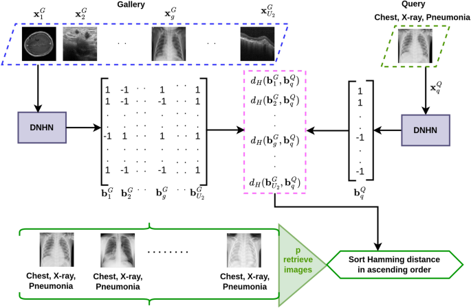
MODHash aims to learn \(F(\cdot )\) on a image pair \(\textbf{x}_{i}^{\mathfrak {T}}~ \text {and} ~ \textbf{x}_{j}^{\mathfrak {T}}\) in a supervised manner such that \(d_H(\textbf{b}_{i}^{\mathfrak {T}}, \textbf{b}_{j}^{\mathfrak {T}}) \rightarrow 0,d_H(\textbf{b}_{1i}^{\mathfrak {T}}, \textbf{b}_{1j}^{\mathfrak {T}}) \rightarrow 0,d_H(\textbf{b}_{2i}^{\mathfrak {T}}, \textbf{b}_{2j}^{\mathfrak {T}}) \rightarrow 0, d_H(\textbf{b}_{3i}^{\mathfrak {T}}, \textbf{b}_{3j}^{\mathfrak {T}}) \rightarrow 0\) if and only if \(s_{ij}=1\), where \(d_H: \{-1,1\}^{K \times 1} \times \{-1,1\}^{K \times 1} \longrightarrow \mathbb {R}\) represents the Hamming distance between two hash vectors. The variables and symbols are presented in Table 1.
Training procedure
The method consists of the following steps. First, the characteristic classification loss is minimized to get distinct features discriminative of the characteristics. Second, the Cauchy cross-entropy loss is employed on hash code to preserve similarity by minimizing the Hamming distance between hash codes of similar characteristics images. The detailed procedure of these steps is discussed as follows.
Initially, a modified version of AlexNet41 is adapted as the backbone architecture to learn the parameters, which is denoted as \(\texttt {Encoder}(\cdot )\). \(\texttt {Encoder}(\cdot )\) takes an input image \(\textbf{x}_{i}^{\mathfrak {T}}\) and produces a feature vector, denoted as \(\textbf{f}_i \in \mathbb {R}^{1024 \times 1}\).
$$\begin{aligned} \textbf{f}_i = \texttt {Encoder}(\textbf{x}_{i}^{\mathfrak {T}}) \end{aligned}$$
(3)
$$\begin{aligned} \begin{aligned} \texttt {Encoder}(\cdot )&\mapsto \texttt {Conv2D: 64c11w4s2p} \rightarrow \texttt {ReLU} \rightarrow \texttt {MaxPool2D: 3w2s} \rightarrow \texttt {Conv2D: 192c5w0s2p} \rightarrow \texttt {ReLU} \\&\rightarrow \texttt {MaxPool2D: 3w2s} \rightarrow \texttt {Conv2D: 384c3w0s1p} \rightarrow \texttt {ReLU} \rightarrow \texttt {Conv2D: 256c3w0s1p} \rightarrow \texttt {ReLU} \\&\rightarrow \texttt {Conv2D: 256c3w0s1p} \rightarrow \texttt {MaxPool2D: 3w2s} \rightarrow \texttt {Flatten} \rightarrow \texttt {Linear: 1024} \end{aligned} \end{aligned}$$
(4)
\(\texttt {Encoder}(\cdot )\) is derived from the initial part of AlexNet, where the last two Linear: 4096 layers are replaced with a single Linear: 1024 layer. The goal is to represent images using a very low-dimensional latent vector for hash code construction, a single linear layer with significantly fewer nodes than the original AlexNet is included. Additionally, three subsequent sub-networks (discussed in the next subsection) are employed to generate three sub-hash codes, each capturing distinct characteristics and requiring additional model parameters.

An overview of characteristic-specific classification loss and hash code generation. The input image \(\textbf{x}_{i}^{\mathfrak {T}}\) passes through a CNN based network \(\texttt{Encoder}(\cdot )\), and then followed by three sub networks \(\mathtt {net_1}(\cdot ), \mathtt {net_2}(\cdot ),\) and \(\mathtt {net_3}(\cdot )\). \(\lambda , \mu , \nu\) denotes the number of modalities, organs, and diseases available in \(\textbf{X}_{\mathfrak {T}}\). \(\textbf{h}_i\) is the hash codes of \(\textbf{x}_i^{\mathfrak {T}}\). The brown arrows represent the forward pass with the tensor, while the red dotted curves indicate the back-propagation of the characteristic-specific classification loss.
Characteristic-specific classification loss
Consider \(\lambda\) number different modalities, \(\mu\) number of different organs, and \(\nu\) number of different diseases present in \(\textbf{X}_{\mathfrak {T}}\). Three simple networks \(\mathtt {net_1}(\cdot ), \mathtt {net_2}(\cdot ),\) and \(\mathtt {net_3}(\cdot )\) are employed on \(\textbf{f}_i\) for respectively classifying the othercharacteristics. \(\hat{\textbf{y}}_{1i}^{\mathfrak {T}} \in \mathbb {R}^{\lambda \times 1}, \hat{\textbf{y}}_{2i}^{\mathfrak {T}} \in \mathbb {R}^{\mu \times 1}\), and \(\hat{\textbf{y}}_{3i}^{\mathfrak {T}} \in \mathbb {R}^{\nu \times 1}\) are predicted characteristics and \(\textbf{z}_{1i} \in \mathbb {R}^{K_1 \times 1}, \textbf{z}_{2i} \in \mathbb {R}^{K_2 \times 1}\), and \(\textbf{z}_{3i} \in \mathbb {R}^{K_3 \times 1}\) are code features obtained from (5), (6), (7) respectively.
$$\begin{aligned} (\hat{\textbf{y}}_{1i}^{\mathfrak {T}}, \textbf{z}_{1i} )&= \mathtt {net_1}( \textbf{f}_i) \end{aligned}$$
(5)
$$\begin{aligned} (\hat{\textbf{y}}_{2i}^{\mathfrak {T}}, \textbf{z}_{2i} )&= \mathtt {net_2}( \textbf{f}_i) \end{aligned}$$
(6)
$$\begin{aligned} (\hat{\textbf{y}}_{3i}^{\mathfrak {T}}, \textbf{z}_{3i} )&= \mathtt {net_3}( \textbf{f}_i) \end{aligned}$$
(7)
$$\begin{aligned} \mathtt {net_1}(\cdot )&\mapsto \mathtt {Linear:512} \rightarrow (\mathtt {Linear:}\lambda , \texttt{Linear}:K_1) \end{aligned}$$
(8)
$$\begin{aligned} \mathtt {net_2}(\cdot )&\mapsto \mathtt {Linear:512} \rightarrow (\mathtt {Linear:}\mu , \texttt{Linear}:K_2) \end{aligned}$$
(9)
$$\begin{aligned} \mathtt {net_3}(\cdot )&\mapsto \mathtt {Linear:512} \rightarrow (\mathtt {Linear:}\nu , \texttt{Linear}:K_3) \end{aligned}$$
(10)
The above three networks generate two outputs, represented as a tuple. The first component of the tuple provides the characteristic-specific classification output, while the second component represents the characteristic-specific sub-hash code for an image. The hash code length is a user-defined, fixed value, while the number of classes depends on the dataset being used. Thus, the number of characteristic-specific classes and the hash code length are two independent variables. The motivation behind using these types of networks is to generate an accurate hash code representation based on the given information about the number of classes. All three characteristics are treated with equal importance in this work, and hence the identical architecture is used.
Given an input image \(\textbf{x}_{i}^{\mathfrak {T}}\) and its corresponding class labels \(\textbf{y}_{1i}^{\mathfrak {T}}, \textbf{y}_{2i}^{\mathfrak {T}}, ~ \text {and}~ \textbf{y}_{3i}^{\mathfrak {T}}\), the objective of this step is to minimize the classification losses \(J_1(\hat{\textbf{y}}_{1i}^{\mathfrak {T}}, \textbf{y}_{1i}^{\mathfrak {T}}), J_2(\hat{\textbf{y}}_{2i}^{\mathfrak {T}}, \textbf{y}_{2i}^{\mathfrak {T}})\), and \(J_3(\hat{\textbf{y}}_{3i}^{\mathfrak {T}}, \textbf{y}_{3i}^{\mathfrak {T}})\) for three respective characteristics. These losses are evaluated using cross-entropy (CE) loss. The total loss for this step is given by,
$$\begin{aligned} L_1 = \sum _{\textbf{x}_{i}^{\mathfrak {T}} \in \textbf{X}_{\mathfrak {T}}} \left[ J_1(\hat{\textbf{y}}_{1i}^{\mathfrak {T}}, \textbf{y}_{1i}^{\mathfrak {T}})+ J_2(\hat{\textbf{y}}_{2i}^{\mathfrak {T}}, \textbf{y}_{2i}^{\mathfrak {T}})+J_3(\hat{\textbf{y}}_{3i}^{\mathfrak {T}}, \textbf{y}_{3i}^{\mathfrak {T}}) \right] \end{aligned}$$
(11)
The above loss helps generate accurate characteristic predictions and, consequently, hash code generation from \(\texttt {Encoder}(\cdot )\) and the three networks described.
Hash code generation
The \(sign(\cdot )\) function is employed to convert the real valued hash to a binary hash representation. The hyperbolic tangent function \(Tanh(\cdot )\) is used during training to avoid the vanishing gradient22 challenge faced on account of the \(sign(\cdot )\) function. Thus, \(\textbf{h}_i\) is utilized during training instead of \(\textbf{b}_i^{\mathfrak {T}}\).
Three sub-hash codes \(\textbf{b}_{1i}^{\mathfrak {T}} \in \{-1,1\}^{K_1 \times 1}, \textbf{b}_{2i}^{\mathfrak {T}} \in \{-1,1\}^{K_2 \times 1}, \textbf{b}_{3i}^{\mathfrak {T}} \in \{-1,1\}^{K_3 \times 1}\) of \(\textbf{x}_{i}^{\mathfrak {T}}\) can be computed as,
$$\begin{aligned} \textbf{b}_{1i}^{\mathfrak {T}}&= sign(\textbf{h}_{1i}) =sign( Tanh(\textbf{z}_{1i}) \end{aligned}$$
(12)
$$\begin{aligned} \textbf{b}_{2i}^{\mathfrak {T}}&= sign(\textbf{h}_{2i}) =sign( Tanh(\textbf{z}_{2i})) \end{aligned}$$
(13)
$$\begin{aligned} \textbf{b}_{3i}^{\mathfrak {T}}&= sign(\textbf{h}_{3i}) =sign( Tanh(\textbf{z}_{3i})) \end{aligned}$$
(14)
The final hash code \(\textbf{h}_i\) and \(\textbf{b}_i^{\mathfrak {T}}\) can represented as,
$$\begin{aligned} \textbf{b}_i^{\mathfrak {T}}&= sign( \textbf{h}_i)\end{aligned}$$
(15)
$$\begin{aligned} \textbf{h}_i&= [\textbf{h}_{1i}, \textbf{h}_{2i},\textbf{h}_{3i}] \end{aligned}$$
(16)
The final real valued hash code \(\textbf{h}_i \in [-1, 1]^{K \times 1} (K = K_1 + K_2 + K_3)\) of input image \(\textbf{x}_i^{\mathfrak {T}}\) is concatenated by three sub-hash codes \(\textbf{h}_{1i}^m \in [-1, 1]^{K_1 \times 1}\), \(\textbf{h}_{2i} \in [-1, 1]\), \(\textbf{h}_{3i} \in [-1, 1]^{K_3 \times 1}\). The training procedure of this step is illustrated in Fig. 2.
Cauchy cross-entropy loss
Learning the relationship between the manifested HD and semantic similarities is a crucial aspect of the retrieval task. Consider an image pair \(\textbf{x}_{i}^{\mathfrak {T}}\) and \(\textbf{x}_{j}^{\mathfrak {T}}\) and their hash codes \(\textbf{h}_i\) and \(\textbf{h}_j\) to be generated using (16). The Cauchy entropy loss is calculated between \(s_{i,j}\) and \(\hat{s}_{i,j}\) using binary cross-entropy, and is given by,
$$\begin{aligned} L_2&= -[s_{i, j} \log \left( \hat{s}_{i,j}\right) +(1-s_{i, j}) \log \left( 1-\hat{s}_{i,j}\right) ] \end{aligned}$$
(17)
$$\begin{aligned}&= s_{i, j} \log \left( \frac{d(\textbf{h}_i, \textbf{h}_j)}{\gamma } \right) + \log \left( 1 + \frac{\gamma }{d(\textbf{h}_i, \textbf{h}_j)} \right) \end{aligned}$$
(18)
where, predicted semantic similarity \(\hat{s}_{i,j}\) is defined as,
$$\begin{aligned} \hat{s}_{i,j} = \frac{\gamma }{\gamma + d_H(\textbf{h}_i, \textbf{h}_j)} \end{aligned}$$
(19)
where, \(\gamma\) is the scale parameter for Cauchy probability distribution22 and the Hamming distance between \(\textbf{h}_i\) and \(\textbf{h}_j\) is \(d_H(\textbf{h}_i, \textbf{h}_j)\). The idea of (19) is that if predicted semantic similarities increase, the Hamming distance (HD) decreases, and vice versa.
Overall loss
The overall loss is computed as,
$$\begin{aligned} L = L_1 + L_2 + \alpha L_3 \end{aligned}$$
(20)
where, \(\alpha\) is scale hyperparameter of the quantization loss (\(L_3\)) of a hash code \(\textbf{h}_i\), which is defined by,
$$\begin{aligned} L_3 = \sum _{i} \Vert \textbf{h}_i – \textbf{b}_i^{\mathfrak {T}}\Vert _2 \end{aligned}$$
(21)
By minimizing L, thereby updating the parameters of \(\texttt {Encoder}(\cdot )\), \(\texttt {net}_\texttt {1}(\cdot )\), \(\texttt {net}_\texttt {2}(\cdot )\) and \(\texttt {net}_\texttt {3}(\cdot )\). The overall method is outlined in Algorithm 1.

The pseudo code for the overall training pipeline of our method to learn and generate hash codes from images.
