Self-supervised learning reveals clinically relevant histomorphological patterns for therapeutic strategies in colon cancer

Ethics statement

Our research complies with all relevant ethical regulations. The study protocol was approved by Applied Bioinformatics Laboratories of New York University Grossman School of Medicine and the Department of Surgery of Leiden University Medical Center. The analyses were performed using anonymized archival material, not necessitating additional informed consents. Data from TCGA-COAD was open-accessed, ensuring patient anonymity without risk of patient identification. All institutions contributing annotated biospecimens provided documentation to the TCGA, and have obtained ethical approvals to use the sample and data according to the human subjects protection and data access policies in TCGA program. Archival material derived from the AVANT-trial (BO17920) was performed in accordance with the declaration of Helsinki^30,31. Protocol approval was obtained from the local medical ethics review committees or institutional review boards at participating sites.

Study population

The TCGA-COAD dataset was used for training and extracting features and histologic patterns using SSL. This dataset consisted of 451 WSIs from 444 unique patients²⁹ with matched genetic and transcriptomic information. We excluded duplications and WSIs with erroneous resolution that were not suitable for the analyses (i.e. only several kilobytes in size). The final TCGA training set included 435 WSIs from 428 patients with a diagnosed pathological TNM-stage I-IV colon carcinoma (333 alive, 94 dead, and 1 missing vital status). We referred to the source population which TCGA-COAD representing as the “standard-of-care” group, contrasting it with the clinical trial external test data described below.

As external dataset we leveraged a study comprising 1213 colon cancer patients with available diagnostic H&E WSIs (one WSI per patient) as part of the clinical Bevacizumab-Avastin® adjuVANT (AVANT) trial^30,31. Bevacizumab, a VEGF monoclonal antibody, had initially been shown to improve the OS in patients with metastatic colon cancer when jointly used with the standard chemotherapy³³. In the phase III AVANT trial, with an intent-to-treat population of 3451 patients, an open-label design was used³⁰. Patients were randomly assigned in a 1:1:1 ratio to three different treatment regimens: FOLFOX-4 (intravenous 5-fluorouracil/folinic acid plus oxaliplatin), bevacizumab-FOLFOX4, and bevacizumab-XELOX (oral capecitabine plus intravenous oxaliplatin)³⁰. The study aimed to investigate whether adding bevacizumab to the standard oxaliplatin-based adjuvant chemotherapy could improve DFS among patients with stage II-high risk and III colon cancer³⁰. However, the trial was prematurely terminated due to the serious adverse effect on the patient’s OS in the bevacizumab-treated group³⁰. The AVANT trial was chosen also due to the previously studied potential correlation of VEGF, the stromal compartment (e.g. TSR), and patient prognosis^31,38,43. For a detailed overview of the trial and patient characteristics, see Zunder et al.³¹.

Given the unique treatment regimen of bevacizumab and its adverse effect in non-metastatic colon cancer, as also proven by a predecessing clinical trial, the NSABP protocol C-08 trial⁶³, we decided to primarily validate OS prediction, trained in the TCGA-COAD, within the control group who only received FOLFOX-4 (without bevacizumab) and refer to it as the “AVANT control group”. Subsequently, as several phase III trials had demonstrated that FOLFOX and XELOX are comparable in the context of metastatic colorectal cancer^33,34,35, we thus combined the bevacizumab+FOLFOX-4 and bevacizumab+XELOX groups into a unified “AVANT-experimental group” and conducted a separate analysis to predict OS within the bevacizumab-treated patients.

Data pre-processing

Tissue segmentation and image tiling

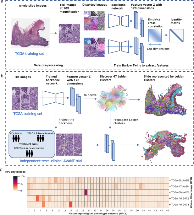
We used the preprocessing methods described in our previous study⁶⁴. Tissue areas in WSIs were segmented against background at 10x magnification level (pixel size approximate 1.0 um). WSIs were divided into non-overlapping image tiles of size 224×224 pixels. The selection of a 10x magnification was based on two key considerations. Firstly, it aligns with the standard magnification utilized by pathologists during microscopic assessments in clinical practice. Secondly, we conducted visual inspections of tiles at 20x, 10x, and 5x magnifications, and found that tiles at 10x magnification provided an optimal balance of capturing sufficient detail while also offering a reasonably sized overview of the morphological structure. In addition, to overcome the variability of color stains from different scan facilities in the TCGA and AVANT cohorts, we further applied the color normalization⁶⁵. In total, we obtained 1,117,796 tiles in the TCGA training set (i.e. TCGA-COAD), and 4,827,055 tiles in the AVANT external test set (AVANT-COAD, consisting of the standard and experimental treatment groups).

Extracting image features using Barlow Twins

We trained the SSL Barlow Twins feature extractor based on 250,000 image tiles randomly selected from the TCGA-COAD dataset. The Barlow Twins extracted unique latent vectors (128 dimension) from the preprocessed image tiles in TCGA. The model is based on ResNet-like architecture consisted of several ResNet layers and one self-attention layer²³. In essence, the Barlow Twins calculates the cross-correlation matrix between the embedding outputs of two identical twin networks, both fed with distorted versions of the same image tile²⁵. It is optimized to make the correlation matrix close to the identity matrix²⁵. We used the batch size of 64 trained on a single NVIDIA® Tesla V100 GPU for 60 epochs. The Barlow Twins feature extractor was frozen after the training and used to project image tiles into latent representation in the entire TCGA training set.

To facilitate the downstream analysis, we also applied five-fold CV partition in the TCGA-COAD training set on patient level balanced the on AJCC TNM stage, OS outcomes (i.e. death or censor), and binned survival time categories.

Leiden community detection algorithm

The Leiden clustering algorithm is a graph-based clustering algorithm that aims to identify distinct communities or clusters within graph data⁶⁶. In brief, it optimizes the modularity function (Eq. 1), in such way to maximize the difference between the actual number of edges and the expected number of edges in a community⁶⁶. This modularity function also includes a resolution parameter γ, with higher values leading to more clusters and lower values leading to fewer clusters. Leiden clustering is initiated by assigning each node in the graph to its own individual cluster, treating them as separate communities, then iteratively optimizes the modularity function by moving a node from its current cluster to a neighboring cluster or by merging clusters until the algorithm converged and revealing distinct communities or clusters. We employed the Leiden clustering in a particular workflow. We began by constructing a neighborhood graph using the K = 250 nearest neighbors from a pool of 200,000 randomly selected latent image vectors from a training set. Subsequently, we applied the Leiden algorithm to identify clusters within this neighborhood graph. These cluster labels were then propagated to each individual image tile across the entire dataset, once more utilizing the K-nearest neighbors approach.

Modularity measures the difference between the actual number of edges in a community and the expected number of such edges. e_c denotes the actual number of edges in community c and the expected number of edges is expressed as \(\frac{{K}_{c}^{2}}{2m}\), where K_c is the sum of the edges of the nodes in community c and m is the total number of edges in the network. γ is the resolution parameter, with higher values leading to more clusters and lower values leads to fewer clusters.

Identification of HPCs

We identified HPCs as clusters obtained from the Leiden community detection algorithm operated on 128-dimensional image features extracted through the Barlow Twins encoder. The Leiden method was also used for quality control to eliminate artifacts and underfocused image tiles. Quality control was carried out after training the Barlow Twins and extracting image features. In the overall process, we initially generated a substantial number of Leiden clusters. Next, we visually examined sample image tiles from each cluster and removed clusters exhibiting artifacts such as air bubbles, foreign objects, etc., or those containing under-focused images. In particular, within the training set of a randomly selected CV fold (fold 0), we randomly selected 200,000 latent image vectors to generate Leiden clusters. We obtained 125 clusters at a high resolution of γ = 6. The Leiden labels were propagated into the entire TCGA set using again the K-nearest neighbors method. Next, we inspected randomly selected sample tiles (N = 32) from each cluster and identified 12 clusters containing predominately artifacts or underfocused images. Image tiles labeled by these 12 clusters were subsequently removed from the further analyses. The HPCs were newly derived in this cleaned dataset by re-running the Leiden clustering. Optimization of the HPCs was conducted using primarily unsupervised methods and secondarily confirmed using supervised methods. Importantly, both the two approaches converged on the same optimal Leiden resolution, as elaborated below.

Optimization of HPCs using unsupervised methods

Leiden resolutions (i.e. γ = 0.4, 0.7, 1.0, 1.5, 2.5, and 3.0) were optimized using three unsupervised statistical tests: the Disruption score, Silhouette score, and Daves-Boundin index. Due to the potentially high variance in data from the different institutions in the TCGA, all three scores were weighted by the mean percentage of the institution presence in each cluster. We consistently identified the optimal Leiden resolution as 1.5 through the three aforementioned statistical tests (Supplementary Fig. 1a).

Optimization of HPCs and the prediction of OS using Cox regressions with L2 regularization

To identify optimal HPC configurations and their associations with patient OS, we trained L2 regularized Cox regressions for OS prediction using 5-fold CV. The Cox regressions were trained separately among standard-of-care colon cancer patients (i.e. TCGA-COAD) and among the AVANT-experimental group.

OS prediction in the standard-of-care group

Prediction of OS from HPCs among the standard-of-care group was trained within TCGA-COAD using 5-fold CV and tested in the independent AVANT control group. Specifically, for each CV fold within TCGA-COAD, we began by generating a range of Leiden clustering configurations at various resolutions, including γ values of 0.4, 0.7, 1.0, 1.5, 2.5, and 3.0, using the method described earlier. Next, at each Leiden resolution, we calculated the compositional representation of HPCs for each WSI (see Main Fig. 1c), followed by a center-log-ratio transformation (Eq. 2). This transformation was designed to mitigate inter-dependencies among HPCs, ensuring that the independence assumptions required for subsequent Cox regression analysis were met. The L2 regularized Cox regressions were then trained at the patient level, with one WSI per patient considered. At each Leiden resolution, we performed a multivariable L2 regularized Cox regression, incorporating all center-log-ratio-transformed HPCs specific to that resolution. We finetuned L2 regularizer (alpha) through an iterative process involving 50 steps, spanning the alpha range from 10⁻⁴ to 10⁴. This sequence of steps was repeated across all five cross-validation folds. The optimal Leiden resolution and L2 regularizer was selected based the CV C-index.

Through this optimization process, the optimal Leiden resolution was determined to be 1.5, and the L2 regularizer alpha was fixed at 0.1842. Of the note, this optimal Leiden resolution of 1.5 concurred with the result from the unsupervised approaches. An HPC-based classifier was determined by the median predicted hazard obtained in the TCGA-COAD. Once the Cox model is optimized, we evaluated the final model performance in the external test set consisting of the AVANT-standard care group. First, the 47 HPCs were integrated into the AVANT-standard care group by employing the K-nearest neighbors method (K = 250), where each AVANT tile’s HPC label was determined based on the majority votes from its nearest neighbors in the TCGA training set. Next, the trained Cox model, with optimized regularization and parameter estimates for the HPCs, was then applied to the AVANT-standard care group to test the prediction of OS (Supplementary Fig. 3b).

Furthermore, employing the same CV method, we trained a clinical baseline model on OS in TCGA-COAD using L2 regularized Cox regression incorporating age, sex, TNM staging, and TSR as predictors. We observed a c-index of 0.58 (bootstrap 95% CI = 0.49-0.67) in the independent AVANT-standard care group and the model-based risk classifier did not reach the statistical significance level (Supplementary Fig. 3c). This baseline model illustrates a simulation of decision-making in clinical practice as control, using the most readily available and relevant clinical and demographic variables. Our HPC-based model outperformed this clinical baseline model. In addition, we explored whether the HPC-based classifier add additional prognostic value to the existing important clinical predictors. We fitted an ordinary multivariable Cox regression within the external AVANT-standard care group, including HPC-based classifier, sex, age, TSR, and AJCC TNM stage (Main Fig. 4a).

The center-log-ratio transformation (clr) calculates the natural logarithm of the ratio (x_i) of compositional data for a specific cluster (C_i) to the geometric mean (g) of the compositional data across all clusters. The compositional data (x_i) is obtained by dividing the counting of tiles in cluster C_i by the total number of tiles in each WSI. The geometric mean (g) is computed by multiplying the compositional data values (x_i) for each cluster (C_i), ranging from i = 1 to n (where n is the total number of clusters), and raising the resulting product to the power of \(\frac{1}{n}\).

OS prediction in the AVANT-experimental group

Bevacizumab, a unique intervention investigated in the AVANT trial, was unlikely accessed by patients from the TCGA-COAD cohort. Considering the significant poor prognostic outcome associated with bevacizumab in non-metastatic colorectal cancer, we postulated that the relationship between HPCs on OS might be influenced by this intervention. Furthermore, we hypothesized that estimates of HPCs on OS trained from the general COAD population, such as TCGA, might not be applicable to bevacizumab-treated patients.

To address these hypotheses, we conducted a separate 5-fold CV estimating the relationship between HPCs and OS within the bevacizumab-treated patients (AVANT-experimental group). Similarly, we generated 5-fold train-validation split stratified by TNM stage and survival time. We used the same sets of HPCs obtained at the previously optimized Leiden 1.5 resolution. Similarly, we modelled the center-log-transformed compositional data of HPCs on OS using Cox regressions with L2 regularization. We fine-tuned the L2 regularizer specifically for AVANT-experimental group. The model performance of HPCs on OS prediction was evaluated using c-index in the 5-fold CV validation sets (Supplementary Fig. 3d).

To understand the importance of each HPC on OS, we employed SHAP values⁶⁷. SHAP values measure the marginal contribution of a HPC towards the predicted OS, considering all possible combinations of features. We highlighted top 20 important HPCs favoring and hindering survival for both standard-of-care and AVANT-experimental treated COAD patients.

Interpretation of HPCs

Plotting HPCs using UMAP and PAGA plot

We applied UMAP dimensionality reduction⁶⁸ to TCGA-COAD tile vector representations (128 dimensional vectors), color-coded by 47 HPC IDs using optimized Leiden clustering configuration from the prior step. Next, we generated a PAGA plot where each HPC is a node connected by lines based on vector similarity. Pie charts within each HPC node showed annotated tissue type percentages annotated independently by three experts (ASLPC, JHJMvK, and MP) (see below). We analyzed this plot to identify and describe significant interconnected clusters (Main Fig. 2b). Based on the PAGA plot, we also defined the “super-clusters” (Main Fig. 2c) according to the interconnections among HPCs and tissue composition.

Pathologist assessment of HPCs

Histopathological assessment and characterization of HPCs

The histomorphological features of 47 HPCs derived in TCGA training set were comprehensively and independently analyzed by two expert pathologists (ASLPC and JHJMvK) and one medical researcher (MP). The analysis was exclusively conducted using image tiles and the assessors were kept blinded to results from other analyses. Specifically, we randomly selected a set of 32 tiles from each HPC within TCGA and each individual tile was examined with specific focus on tumor epithelium, tumor stroma, and immune cells. Attention was also paid to general tumor differentiation grade, tumor stromal amount, stromal classification, i.e. aligned or disorganized, stromal neovascularization or other notable patterns (e.g. dysplastic tissue, fatty tissue, muscle tissue fibers, blood vessels, erythrocytes, etc.)^3,43,59. Each assessor evaluated the tissue composition based on 32 randomly selected tiles per HPC, providing an average tissue composition for each HPC. In cases of conflicting tissue annotations, the assessors carried out discussions to achieve consensus. In addition, a short label was given to each HPC based on tissue annotation either according to the first and second predominant tissue types and patterns (e.g. “aligned stroma – well differentiated tumor epithelium”), or as the single most dominant tissue type covering ≥70% area of an average tile (e.g. “necrotic”). The tissue description, composition, and short labels of all 47 HPCs were displayed in Supplementary Table 1.

Assessment of HPC consistency within and across TCGA and AVANT cohorts We performed various qualitative and quantitative analyses to evaluate the within-cluster and between-cluster heterogeneity of HPCs, as well as their transferability from TCGA to AVANT cohorts. Initially, qualitative visual assessments were independently conducted by three experts (ASLPC, JHJMvK, and MP) to evaluate the concordance within and discordance between HPCs. This evaluation followed the established protocol for tissue type analysis, utilizing the previously randomly selected 32 tiles per HPC. The assessors noted consistent histomorphological patterns within HPCs and diverse patterns across various HPCs.

In addition, we conducted quantitative objective tests within TCGA and AVANT tiles separately to determine if the learned morphological features of the HPCs could be replicated by human eyes. We displayed three rows, each containing five tiles, which is referred to as a “question”. Among these rows, two belonged to the same HPC, while the third row, also referred to as the “odd HPC”, were tiles randomly selected from a different HPC. All example tiles were randomly selected within each HPC. The researcher (MP) was required to identify the “odd HPC”, and upon doing so, the next question was presented (example shown in Supplementary Fig. 2). In order to calculate the success rate, we ran 50 questions per HPC and we repeated the experiment for all 47 HPCs. The test was conducted on a closed website accessible through login and was conducted separately for tiles randomly selected from TCGA and AVANT. The conducted experiment exhibited an average completion time of under 10 seconds per question. The success rate was determined for each HPC by dividing the number of incorrect answers by the total number of questions (50 questions per HPC). We hypothesized that most HPCs would be distinguishable. However, some HPCs may be challenging to differentiate due to tissue similarities, either within the same super-cluster or through similar tissue morphology (e.g., muscle tissue and tumor stroma). The results showed that HPCs in close proximity to each other in the PAGA or belonging to the same super-cluster were indeed more prone to being mistaken.

To validate whether HPCs derived from the TCGA training set generalized well in the external AVANT test set, three assessors (ASLPC, JHJMvK, and MP) independently carried out visual examination of tissue characteristics in 32 randomly selected tiles from each HPC in both the AVANT trial and the TCGA set, comparing their histomorphological features regarding tissue types and composition established in the previous step. Assessors confirmed that the consistent and meaningful patterns, as learned by the Barlow Twins, could be replicated across other clinical cohorts like the AVANT trial. To validate our observation, we compared the objective test results between TCGA and AVANT, focusing on the overlap in both misclassified and correctly classified HPCs across the datasets.

Linkage between survival-related HPCs, immune landscape, and gene expression data

We calculated Spearman correlations between HPCs and RNASeq-derived immune features from TCGA-COAD data, correcting for false discovery rate (0.05) using Benjamini-Hochberg correction. We created bi-hierarchical clusters for immune features and top 20 significant HPCs linked to OS in both standard-of-care and AVANT-experimental groups. Clustering was based on correlation coefficients using Euclidean distance and Ward’s aggregation.

In addition, we performed GSEA to explore the potential associations between HPCs and the major cancer hallmark pathways, as previously described⁶⁹. The analysis was conducted within 282 TCGA-COAD patients with available gene expression data for 20,530 genes. For each HPC, we calculated the Spearman correlation coefficients with the expression data of these 20,530 genes and sorted the resulting correlation coefficients to rank the genes in a descending order. Subsequently, enrichment scores for 50 major cancer hallmark pathways, as defined by the “MSigDB_Hallmark_2020” gene set⁵⁸, were computed for each HPC based on the generated ranked gene list. A positive enrichment score indicated higher composition of a HPC was associated with gene enrichment in a pathway and a negative value suggested higher composition of a HPC was associated with underrepresentation of a pathway. We plotted the cancer hallmark enrichment scores for the top 20 important HPCs related to OS, for both the general and experimental treatment groups. We set a significance level of 0.01 of the false discovery q value. The analysis was conducted using the gseapy (1.0.4) Python package. Two-way hierarchical clustering was based on the Euclidean distance of the enrichment scores and Ward’s aggregation method.

Lastly, we created a Supplementary Table 2 to grant a detailed overview of the significant HPCs associated with OS, including the direction of the association (worse or better OS) for both treatment groups (TCGA and AVANT standard, or AVANT-experimental) and in-depth histopathological analyses potentially explaining these associations with appropriate references.

Reporting summary

Further information on research design is available in the Nature Portfolio Reporting Summary linked to this article.