Knowledge-guided diffusion model for 3D ligand-pharmacophore mapping

Dataset construction

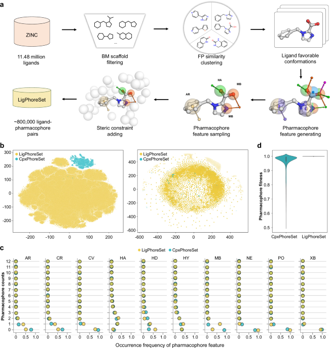
We constructed two 3D ligand-pharmacophore pair datasets, CpxPhoreSet and LigPhoreSet, for LPM learning, by using the enhanced version of AncPhore²³. CpxPhoreSet was established by analyzing a total of 19,443 protein-ligand complex structures collected in PDBBind (version 2020)^47,48. We followed a time-split scheme¹⁴ and divided PDBBind into train (16,379 entries), validation (968 entries), and test (363 entries) sets. The train and validation set were used to establish the CpxPhoreSet and the remaining test set was used for performance evaluation. For each complex structure, AncPhore was used to generate one pharmacophore model considering 10 pharmacophore feature types (HD, HA, MB, AR, PO, NE, HY, CV, CR, and XB) and exclusion spheres (EX) according to protein-ligand interactions. These models with less than 3 features and more than 15 features were disregarded. The retained pharmacophore models, along with ligand conformations, constituted the CpxPhoreSet, encompassing a total of 15,012 ligand–pharmacophore pairs.

We started LigPhoreSet construction with ~11.48 million ligands (with molecular weights less than 800 and LogP less than 5) obtained from the In-Stock subset of the ZINC20 database⁴⁹ (downloaded in May, 2023). After removing duplicates, multiple components, and unidentifiable SMILESs using the RDKit software, the remaining ligands were clustered based on Bemis–Murcko scaffold⁵⁰ rules. From each ligand cluster, a representative ligand was randomly chosen. These selected ligands underwent further filtration based on Morgan fingerprint⁵¹ similarity (with a radius of 2) to ensure a broad but nonredundant diversity of ligand chemotypes. Then, each of these filtered ligands generated a corresponding, energetically favorable 3D conformation using the RDKit MMFF force field. Next, the pharmacophore models for all ligand conformations are generated as follows: (1) generating initial pharmacophore models by considering 10 pharmacophore feature types (identical to those used for CpxPhoreSet) for all 3D ligand conformations; (2) retaining the pharmacophore models bearing at least 2 features among MB, HA, HD, AR, NE, or PO; (3) sampling three pharmacophore models with different pharmacophore feature combinations for each ligand conformation; (4) generating exclusion spheres as steric constraints via a pseudo-receptor manner, with exclusion spheres introduced around the ligand conformation at distances ranging from 3 Å to 5 Å. We finally obtained a version of LigPhoreSet comprising 840,288 ligand-pharmacophore pairs derived from 280,096 ligands. To facilitate initial model training and hyperparameter search, we randomly extracted a subset from LigPhoreSet, containing 84,030 samples and 28,010 ligands.

Problem formulation

Generally, the 3D ligand-pharmacophore mapping (LPM) task is to identify a reasonable ligand conformation that maximally matches with a given pharmacophore model. Given the 3D structure of the pharmacophore \({G}_{p}\) and an initial ligand conformation \({G}_{l}\), the LPM model predicts a ligand conformation that satisfies the pharmacophore constraints.

where \({G}_{p}\), \({G}_{l}\) and \({\widehat{G}}_{l}\) represent the 3D representations of the input pharmacophore model, the input ligand conformation and the generated ligand conformation, respectively. The generated ligand conformation \({\widehat{G}}_{l}\) shares the same chemical structure with \({G}_{l}\) and only differs in conformation.

The LPM problem treated by diffusion-based generative modeling

To solve the LPM problem, we need to approximate the conditional probability density of ligand binding conformation \(P({\widehat{G}}_{l}|{G}_{p},{G}_{l})\). In general, the gradient of the probability density \(\nabla P({\widehat{G}}_{l}|{G}_{p},{G}_{l})\) is called the score function. Song and Ermon introduced score-based generative modeling to learn this score function from data and to generate samples with Langevin dynamics⁵². Given an initial sample \({\widehat{G}}_{l,0}\) from any prior distribution \(\pi ({\widehat{G}}_{l,0})\) (e.g., Gaussian distribution), Langevin dynamics is incorporated to perform denoising using the following iterative update:

where \(\epsilon\) is the step size and \(T\) is the number of iterations. \({z}_{t}\) is the sample noise from \({{{\mathcal{N}}}}({{\mathrm{0,1}}})\). \({\widehat{G}}_{l,0}={G}_{l}\) is the input ligand conformation and \({\widehat{G}}_{l,T}={\widehat{G}}_{l}\) is the predicted ligand conformation. Under certain modest conditions^53,54, and with sufficiently small step size \(\epsilon\) and large \(T\), the distribution of \({\widehat{G}}_{l,T}\) will approximate the true distribution of ligand binding conformation \({P}_{{data}}({G}_{l}^{*}|{G}_{p},{G}_{l})\), where \({G}_{l}^{*}\) represents an optimal ligand conformation.

In this paper, we proposed a score-based diffusion model DiffPhore, to iteratively generate the ligand conformation \({\widehat{G}}_{l}\). Specifically, the denoising probability can be formulated as \({P}_{\sigma }({G}_{l,t}|{G}_{l}^{*},{G}_{p})={{{\mathcal{N}}}}({G}_{l,t}|{G}_{l}^{*},{\sigma }^{2}I)\) given the ligand structure \({G}_{l}^{*}\). \({G}_{l,t}\) stands for the perturbed data point at step \(t\). Thus, the perturbed data distribution \({P}_{\sigma }({G}_{l,t}{{|G}}_{p},{G}_{l})=\int {P}_{{data}}({G}_{l}^{*}|{G}_{p},{G}_{l}){P}_{\sigma }({G}_{l,t}|{G}_{l}^{*})d{G}_{l}^{*}\). We consider a sequence of decreasing noise scales \({{\left\{{{{{\rm{\sigma }}}}}_{{{{\rm{t}}}}}\right\}}^{{{{\rm{T}}}}}}_{{{{\rm{t}}}}=1}\) (\({{{{\rm{\sigma }}}}}_{1} > {{{{\rm{\sigma }}}}}_{2} > \ldots > {{{{\rm{\sigma }}}}}_{{{{\rm{T}}}}}\)). DiffPhore introduces a score network^52,55 \({CFGenerator}({G}_{l,t},{G}_{p},t)\) to estimate the score function at each noise level \({\sigma }_{t}\). Thus, the training loss of this score network is

As for the generation stage, DiffPhore sequentially performs \(T\) steps of Langevin MCMC to obtain a reasonable ligand conformation mapped with the given pharmacophore.

Where \({\epsilon }_{t-1}\) is the step size at \(t-1\). In the next section, we will explain the detailed implementations of the above generative modeling framework.

DiffPhore architecture

To iteratively generate reasonable ligand conformations given the pharmacophore, DiffPhore adopts the following three main components, including a knowledge-guided LPM representation encoder (\({LPMEncoder}\)), a conformation generator (\({CFGenerator}\)), and a calibrated conformation sampler (\({CCSampler}\)). As the input of the score network, the LPM representation leverages pharmacophore principles to characterize 3D mapping relationships of the ligand conformation-pharmacophore pairs. The conformation generator takes LPM representations as inputs to iteratively search ligand conformations to fit with a pharmacophore model, continuing until the maximum alignment is achieved. The calibrated conformation sampler is designed to eliminate the exposure bias of the iterative conformation search process.

Knowledge-guided LPM representations

Accurately representing LPMs is the prerequisite for successfully performing the task of fitting ligand conformations to pharmacophores. We proposed a heterogenous geometric graph \({G}_{t}\) to characterize LPMs in the 3D space,

where \({G}_{l,t}=\{{{{{\mathcal{V}}}}}_{l},{{{{\rm{x}}}}}_{{{{\rm{t}}}}},{{{{\mathcal{E}}}}}_{l},{{{{\rm{V}}}}}_{l}\}\) is a ligand graph at the t-th step, \({G}_{p}=\left\{{{{{\mathcal{V}}}}}_{p},{{{{\rm{x}}}}}_{{{{\rm{p}}}}},{{{{\mathcal{E}}}}}_{p},{{{{\rm{V}}}}}_{p}\right\}\) is a pharmacophore graph, and \({G}_{{lp}}\) is a bipartite graph (Fig. 2b; see details in Supplementary Methods). \({{{{\mathcal{V}}}}}_{l}\) and \({{{{\rm{x}}}}}_{{{{\rm{t}}}}}\) stand for the ligand atoms and their 3D coordinates. \({{{{\mathcal{E}}}}}_{l}\) represents the covalent bonds as well as unbonded edges within 5 Å in the ligand. \({{{{\mathcal{V}}}}}_{p}\) and \({{{{\rm{x}}}}}_{{{{\rm{p}}}}}\) represent the pharmacophore points and their 3D coordinates, respectively. \({{{{\mathcal{E}}}}}_{p}\) denotes the connections between each pair of pharmacophore features, and connections of each exclusion sphere to the nearest pharmacophore point in \({{{{\mathcal{V}}}}}_{p}\). \({{{{\rm{V}}}}}_{l}=\{{{{{\rm{v}}}}}_{{ij}}\left|i,j\in {{{{\mathcal{V}}}}}_{l}\right.\}\) and \({{{{\rm{V}}}}}_{p}=\{{{{{\rm{v}}}}}_{{j}^{{\prime} }{k}^{{\prime} }}\left|{j}^{{\prime} },{k}^{{\prime} }\in {{{{\mathcal{V}}}}}_{p}\right.\}\) are vectors connecting the neighboring nodes in \({G}_{l}\) and \({G}_{p}\), respectively.

The bipartite graph \({G}_{{lp}}=\{{{{{\mathcal{V}}}}}_{l},{{{{\mathcal{V}}}}}_{p},{{{{\mathcal{E}}}}}_{{lp}},{{{{\rm{V}}}}}_{{lp}},{{{{\rm{N}}}}}_{{lp}}\}\) is exploited to describe the ligand-pharmacophore matching relations, where \({{{{\mathcal{E}}}}}_{{lp}}\) connects each ligand atom to all the pharmacophore feature points, \({{{{\rm{V}}}}}_{{lp}}=\{{{{{\rm{v}}}}}_{i{j}^{{\prime} }}\left|i\in {{{{\mathcal{V}}}}}_{l},{j}^{{\prime} }\in {{{{\mathcal{V}}}}}_{p}\right.\}\) and \({{{{\rm{N}}}}}_{{lp}}=\left\{{{{{\rm{n}}}}}_{i{j}^{{\prime} }}\left|i\in {{{{\mathcal{V}}}}}_{l},{j}^{{\prime} }\in {{{{\mathcal{V}}}}}_{p}\right.\right\}\) are the pharmacophore type and direction matching vectors, respectively. We detail the featurization and implementation of \({G}_{l,t}\), \({G}_{p}\) and \({G}_{{lp}}\) in Supplementary Methods.

Diffusion-based conformation generator

Given the LPM representations \({G}_{t}\) at random time \(t\), the generator aims to predict the conformations \({\hat{{{{\rm{x}}}}}}_{{{{\rm{t}}}}-\Delta {{{\rm{t}}}}}\) at the former step, given by

Since the degrees of freedom in 3D coordinates are significantly higher than needed, the ligand conformation here is represented by a combination of translations, rotations, and changes to torsion angles. The ligand conformation space can be formulated as an \(\left(m+6\right)\)-dimensional submanifold, \(m\) is the number of rotatable bonds, and 6 refers to the roto-translations¹³. More specifically, the ligand conformation space can be formally defined as:

where \({\mathbb{P}}\) is the product space of 3D translation group \({{\mathbb{T}}}^{3}\), 3D rotation group \({SO}\left(3\right)\) and changes in torsion angles \({SO}{\left(2\right)}^{m}\), \(A\) stands for the total transformation with respect to an element \(g=({{{\rm{r}}}},{{{\rm{R}}}},{{\theta }})\) in the product space \({\mathbb{P}}\), and \({A}_{{tr}},{A}_{{rot}},{A}_{{tor}}\) refer to the actual translation, rotation, and torsion angle transformations. To reduce the prediction complexity, we formulate the prediction task as the learning of the change directions (or scores) in the ligand translation (\({{{\rm{\alpha }}}}\)), rotation (\({{{\rm{\beta }}}}\)), and torsion angles (\({{{\rm{\gamma }}}}\)) instead:

The scores (\({{{\rm{\alpha }}}},{{{\rm{\beta }}}},{{{\rm{\gamma }}}}\)) correspond to the gradient estimates of the translation (\({p}_{t}^{{tr}}\)), rotation (\({p}_{t}^{{rot}}\)) and torsion angle (\({p}_{t}^{{tor}}\)) diffusion kernels, which follow Gaussian distribution, IGSO(3) distribution⁵⁶ and the wrapped normal distribution⁵⁷, respectively. The corresponding gradients (e.g., \(\nabla {p}_{t}^{{tr}}\left(\Delta {{{{\rm{r}}}}}_{0\to {{{\rm{t}}}}} | 0\right)\) can be easily calculated in advance¹³.

The SE(3)-equivariant conformation generator comprises the embedding, update, and output modules (Supplementary Fig. 3a). The update module consists of \(L\) message-passing layers, each with intra- and inter-graph update layers. The intra-graph layer extracts the topological features of the ligand and the pharmacophore separately; the inter-graph layer performs the feature fusion between two graphs, establishing deep representations of the ligand-pharmacophore interactions. Finally, the output module predicts the change directions in the ligand translation (\({{{\rm{\alpha }}}}\)), rotation (\({{{\rm{\beta }}}}\)), and torsion angles (\({{{\rm{\gamma }}}}\)).

Initially, the embedding module processes input ligand and pharmacophore graphs as well as cross-edges between them, and integrates the random diffusion time (\(t\)) into the graph features (Supplementary Fig. 3b; see details in Supplementary Methods). This yields the initial embeddings for ligand (\({h}_{l}^{0},\)\({e}_{l}\)) pharmacophore (\({h}_{p}^{0},{e}_{p}\)) and cross edges (\({e}_{{lp}}\)). Since all the computations of the conformation generator correspond to a specific step, we omit the notation \(t\) for the subsequent features for simplicity.

Next, the update module iteratively refines the initial embeddings via message passing layers (Supplementary Fig. 3c), with each layer comprising intra-graph and inter-graph updates. Intra-graph updates compute messages (\({m}_{l,i-{intra}}\) and \({m}_{p,{j}^{{\prime} }-{intra}}\), Eqs. 13–15) to incorporate the information of internal topological structure within each graph. The updates are computed as tensor products of the node features and the spherical harmonic representations of neighboring edge vectors, weighted by the edge embedding \({e}_{{ij}}\), the outgoing \({h}_{j}\) and the incoming node features \({h}_{i}\).

In the formulas, \({TP}\) denotes the tensor products layer, \({{{{\mathcal{N}}}}}_{i}=\{j|\left(i,j\right)\in {{{{\mathcal{E}}}}}_{l} {\ or\ } {{{{\mathcal{E}}}}}_{p}\}\) stands for neighbor nodes and \(Y\) is the spherical harmonic. \({BN}\) refers to the batch normalization, \(\phi\) stands for a MLP layer, and \(\otimes\) refers to tensor product operation.

The inter-graph layer simulates the ligand-pharmacophore recognition and alignment with the constructed bipartite graph \({G}_{{lp}}\). The pharmacophore type and direction matching vectors are incorporated for the calculation of the inter-graph updates (\({m}_{l,i-{inter}}\), \({m}_{p,{j}^{{\prime} }-{inter}}\)) via similar tensor product layers (Eqs. 16–17). The intra- and inter-graph messages are aggregated to update ligand (\({h}_{l}^{l}\)) and pharmacophore (\({h}_{p}^{l}\)) node embeddings (Eqs. 18–19). All tensor product layers here are implemented using the ‘FullyConnectedTensorProduct’ layer from the E3NN package (see details in Supplementary Methods).

Finally, the output module receives the updated ligand features \({h}_{l}^{L}\) to predict the translation, rotation, and torsion scores w.r.t their diffusion kernels. The translation and rotation are rigid transformations operating on the center of mass of the ligand so that edges between ligand atoms and the center of mass \({{{{\mathcal{E}}}}}_{{ca}}\) are constructed to compute the corresponding scores \({{{\rm{\alpha }}}},{{{\rm{\beta }}}}\) with tensor product layer. Here, \(\psi,\phi\) are MLP layers, and \(\mu (\cdot )\) denotes radical bias embedding of edge length. The vector \({{{{\rm{v}}}}}_{{ca}}\) stands for the 3D vectors from the center of mass to the ligand atom \(a\).

To estimate the torsion score \({{{\rm{\gamma }}}}\), the output layer focuses on the rotatable bonds and the adjacent atoms to predict the corresponding changes in torsion angles. For the torsion score \({{{{\rm{\gamma }}}}}_{{{{\rm{r}}}}}\) of the rotatable \(r\), the output layer performs the tensor product operation between the bond features and the adjacent atom features, given by

where \({{{{\mathcal{N}}}}}_{r}\) is the set of ligand atoms connected with the rotatable bonds. \({T}_{r}\) is a convolutional filter constructed for each rotatable bond \(r\) calculating the tensor product of the spherical harmonic representation of the bond axis \({{{{\rm{v}}}}}_{r}\) (\({Y}^{2}\) here means max level is 2) and the vector \({{{{\rm{v}}}}}_{{rb}}\) from bond center of \(r\) to the atom \(b\). \(\omega\) refers to a MLP layer, \({h}_{r}\) stands for the feature of the rotatable bond \(r\) formed by the involved node features of the incoming node \({h}_{{r}_{{in}}}\) and the outgoing node \({h}_{{r}_{{out}}}\).

The loss function (\({L}_{{diffphore}}\)) of DiffPhore consists of three components corresponding to the translation, rotation and torsion diffusion kernels:

where \({{{{\rm{\alpha }}}}}^{{\prime} },{{{{\rm{\beta }}}}}^{{\prime} }{,{{{\rm{\gamma }}}}}^{{\prime} }\) are the precomputed labels in the training dataset. In this way, the loss function (\({L}_{{diffphore}}\)) enforces the conformation generator to estimate the denoising directions at each step.

Calibrated conformation sampler

Due to the auto-regressive generation fashion, diffusion models usually suffer from the exposure bias, which is caused by the input mismatch between the training and the inference phases. In particular, the conformation generator in the training process takes a perturbed conformation \({{{{\rm{x}}}}}_{{{{\rm{t}}}}}\) as input and the corresponding scores (\({{{{\rm{\alpha }}}}}_{{{{\rm{t}}}}},{{{{\rm{\beta }}}}}_{{{{\rm{t}}}}},{{{{\rm{\gamma }}}}}_{{{{\rm{t}}}}}\)) as the labels. By contrast, the conformation generator is fed with the predicted conformation \({\hat{{{{\rm{x}}}}}}_{{{{\rm{t}}}}}\) during the inference process. To narrow the discrepancy between the training and inference phases, we proposed a calibrated conformation sampler, which mimics the inference process to construct pseudo ligand conformations (\({\widetilde{{{{\rm{x}}}}}}_{{{{\rm{t}}}}}\)) and corresponding scores (\({\widetilde{{{{\rm{\alpha }}}}}}_{{{{\rm{t}}}}},{\widetilde{{{{\rm{\beta }}}}}}_{{{{\rm{t}}}}},{\widetilde{{{{\rm{\gamma }}}}}}_{{{{\rm{t}}}}}\)) for model training (see details in Supplementary Table 3 and Supplementary Methods). The pseudo ligand conformations are estimated based on the denoised data points by DiffPhore and thus alleviating the exposure bias problem.

However, solely relying on these calibrated data points for the model training is infeasible, as the quality of them is inferior to the real data points. Therefore, we utilized an epoch-dependent possibility scheduler to sample the calibrated data as inputs with the probability \({P}_{{epoch}}\) and real data points with the probability (\(1-{P}_{{epoch}}\)). During the training process, the sampling probability \({P}_{{epoch}}\) starts from a small value and gradually increases along with the increment of the training epoch as shown in Eq. 28. where \({p}_{\max },\mu,c\) are hyperparameters (Supplementary Table 11) that balance the utilization of the two types of training data.

The detailed algorithms of \({LPMEncoder}\), \({CFGenerator}\), and \({CCSampler}\), and the model training details can be found in Supplementary Methods and the source codes.

Pharmacophore fitness scorings

To leverage the advantages of DiffPhore in different virtual screening scenarios, we introduced four fitness scorings to evaluate the degree of the alignment between the generated ligand conformations and the reference pharmacophore model. \({DfScore}1\) is a basic scoring function considering pharmacophore feature alignment and exclusion sphere collision, which is calculated using an in-situ max-matching approach as provided in Eqs. 30–32:

where \({V}_{{overlap}}\) represents the total overlap volume between the ligand conformation pharmacophore features (\(L\)) and the reference pharmacophore features (\(P\)). It is calculated as the sum of individual feature overlap volume, considering scaling factors (\({C}_{i}\)), basic weights (\({W}_{i}\)), chemical group weights (\({\lambda }_{i}\)), directional differences (\(f(\theta )\)), tolerance ranges (\({\sigma }_{i,L},{\sigma }_{i,P}\)), the distance of the match pharmacophore pair (\({d}_{i,L-i,P}\)). \({\theta }_{0}\) is set as 0 (the number of root atoms equals 1) or \(\frac{\pi }{3}\) (the number of root atoms larger than 1). \({V}_{{ref}}\) represents the total volume of the reference pharmacophore features. \({V}_{{overlapEX}}\) denotes the sum of volumes where the ligand atoms overlap with reference exclusion volumes. \(\epsilon\) is a maximum tolerance for ligand clashing with pharmacophore, set to 500. \({DfScore}1\) is adopted as the default fitness score for DiffPhore.

Building upon \({DfScore}1\), \({DfScore}2\) includes a bias factor that accounts for the percentage of matched pharmacophore feature pairs, with the aim to consider the tolerance of pharmacophore features. It is calculated by Eq. 33, where \(n\) is the number of matched pharmacophore pairs and \({N}_{{ref}}\) is the total number of reference pharmacophore features. Here, two pharmacophore features are regarded as a matched pair if the distance between them is less longer than their tolerance range.

Recognizing the significance of anchor pharmacophore features in protein-ligand recognition and practical drug discovery²³, we introduced \({DfScore}3\) to specifically measure the alignment of anchor pharmacophore features:

where \({V}_{{Anchor}}\) is the total volume of the anchor features in reference pharmacophore model. \({V}_{{overlapAnchor}}\) is the sum of volumes accounting for the ligand pharmacophore features overlapping with the reference anchor features.

Taking all the factors into consideration, we also proposed a comprehensive fitness score \({DfScore}4\):

In addition, \({DfScore}5\) is specifically designed for target fishing. It further considers the extent to which the number of ligand’s pharmacophore features matches the number of pharmacophore features representing the target.

where \({N}_{{mol}}\) is the count of molecule pharmacophore features.

Baseline setup and implementation

The conformation generation tools, including OpenBabel (version 2.4.1) and Conformator (version 1.2.1), were obtained from their official websites. We utilized the official “AutoPH4” plugin to perform pharmacophore modeling in MOE (version 2020.09) and employed the “Compute | Pharmacophore | Search” functionality for ligand-pharmacophore alignment. The aligned poses in MOE are ranked using the default “rmsdx” metric.

The open-access docking programs, including AutoDock Vina, Uni-dock, SMINA, and GNINA, were implemented following their official source code repositories and instructions. We utilized the “prepare_receptor” and “prepare_ligand” scripts in ADFR toolkit for AutoDock Vina, GNINA, and SMINA to prepare the PDBQT files of protein and ligand structures. As for Uni-dock, its official “unidocktools” was employed. To define the conformation search area, we used a box of \(20 {{{\text{\AA}}}} \times 20{{{\text{\AA}}}} \times 20 {{{\text{\AA}}}}\) centered on the ligand in complex crystal structure for AutoDock Vina and Uni-dock, and utilized the “–autobox_ligand” option with default buffer range (4 Å) for SMINA and GNINA. The number of binding conformations was set to 10 for all docking baselines, with other parameters kept at their default settings.

All these calculations were performed on a Linux Rocky 9.2 operating system, utilizing Intel(R) Xeon(R) Platinum 8378C CPU @ 2.80 GHz and NVIDIA RTX 4090 GPU.

Evaluation metrics

The metrics including Root Mean Square Deviation (RMSD), PoseBusters test validity (PB-Valid), Boltzmann-Enhanced Discrimination of Receiver Operating Characteristic (BEDROC), Enrichment Factor (EF), and Area Under the Receiver Operating Characteristic Curve (AUROC), were used for performance evaluations (see details in Supplementary Methods).

Case study: human glutaminyl cyclases

We used DiffPhore to conduct virtual screening for identifying potential inhibitors for sQC and gQC by employing a substrate-mimicking strategy. First, the binding mode of the tripeptide substrate NH₂-Gln-Phe-Ala-CONH₂ (QFA) with sQC was obtained via our QM/MM calculations. Then, we constructed the pharmacophore modeling from the calculated sQC:QFA complex structure to represent the key binding features of QFA with sQC (Supplementary Fig. 13). Given the pharmacophore model, we then utilized DiffPhore to screen potential hit compounds for sQC against the commercial Vitas-M compound library (https://vitasmlab.biz/) with about 1.4 million compounds available for quick purchase. To efficiently screen the large compound library, we implemented a pharmacophore fingerprint filtering approach, which evaluates the matching context based on the number and types of pharmacophore features, without accounting for their 3D alignment. A pharmacophore fingerprint similarity cutoff of 0.6 was set. To this end, we identified 91,229 ligands from the Vitas-M compound library for subsequent screening by DiffPhore (20 poses generated for each ligand). Through manual inspection, we picked 15 structurally distinct compounds from the top-ranked hits with \({DfScore}1\) for experimental verification.

sQC/gQC/PGP-1 protein expression and purification

We followed the protocols from our previous study⁵⁸ for the expression and purification of human sQC (amino acids 33-361), gQC (amino acids 53-382), and the auxiliary enzyme PGP-1 (amino acids 1-215) (see details in Supplementary Methods).

sQC/gQC/PGP-1 inhibition activity assays

All compounds were tested for their inhibitory activity on sQC, gQC, and PGP-1 in the assay buffer (25 mM Tris-HCl, 150 mM NaCl, 10% glycerol, pH 8.0) as described previously⁵⁸ (see details in Supplementary Methods). All determinations were tested in triplicate.

Thermal shift assays

The sQC or gQC enzymes (5 μM) were first incubated with test compounds (50 μM) or a vehicle at room temperature for 20 minutes in Tris-HCl buffer (25 mM Tris-HCl, 150 mM NaCl, 10% glycerol, pH 8.0). Then, the SYPRO ORANGE dye (10× concentration) was added, and the fluorescence was promptly quantified using a fluorescence quantitative PCR instrument. The temperature was incrementally increased from 30 to 95 °C, rising by 1 °C per cycle. The resulting fluorescence intensity versus temperature was analyzed using GraphPad Prism to determine the melting temperature (T_m) values.

Co-crystallization, data collection, and analysis

The hanging-drop vapor diffusion method was employed for co-crystallization experiments. The purified sQC proteins (8 mg/mL) were incubated with 5/13 (3.9 mM) on ice for 2 h and then centrifuged at 15,777 × g for 10 min to remove insoluble materials. Crystals were grown under the condition: 12−16% (v/v) polyethylene glycol 4000, 0.2 M MgCl₂ and 0.1 M Tris-HCl at pH 8.5. The protein solution was mixed with the reservoir solution at a 1:1 ratio. The crystals were cryoprotected with the mother liquor supplemented with 30% (v/v) glycerol prior to harvesting. Data collection was performed at the BL18U1 beamline at the Shanghai Synchrotron Radiation Facility. The diffraction data were processed using XDS⁵⁹ or AutoXP⁶⁰, followed by structural determination with PHENIX⁶¹ and WinCoot⁶². We utilized the existing crystal structure of sQC (PDB code 3PBB) as the template in the molecular replacement step. The crystal structures of sQC:5 (PDB code 9ISD) and sQC:13 (PDB code 9IVV) are available in the Protein Data Bank.

Reporting summary

Further information on research design is available in the Nature Portfolio Reporting Summary linked to this article.