Infusing structural assumptions into dimensionality reduction for single-cell RNA sequencing data to identify small gene sets

Mathematical notations

Matrices are written in capital bold letters, and vectors in lowercase bold letters. Greek letters are used for denoting model parameters or hyperparameters. Vectors are treated as column vectors. Scalar values are denoted by lowercase letters. In general, \({{{\boldsymbol{X}}}}\in {{\mathbb{R}}}^{n\times p}\) denotes a matrix of n i.i.d. observations (cells) of p variables (genes) sampled from an unknown probability distribution. Observations, i.e., rows of X, are denoted by x₁, …, x_n and the columns of X by x⁽¹⁾, …, x^(p). We define the zero-matrix with n rows and p columns by \({{{{\boldsymbol{0}}}}}_{{{\mathbb{R}}}^{n\times p}}\). Further, by \({\widehat{\mu }}_{{{{\boldsymbol{x}}}}}:= \frac{1}{n}{\sum }_{i = 1}^{n}{x}_{i}\) we denote the sample mean of a vector \({{{\boldsymbol{x}}}}={({x}_{1},\ldots ,{x}_{n})}^{\top }\) and by \({\widehat{\sigma }}_{{{{\boldsymbol{x}}}}}:= \sqrt{\frac{1}{n-1}{\sum }_{i = 1}^{n}{({x}_{i}-{\widehat{\mu }}_{{{{\boldsymbol{x}}}}})}^{2}}\) the corrected sample standard deviation of x. The sample Pearson correlation coefficient of two vectors x, y is denoted by \(\widehat{{{{\rm{cor}}}}}({{{\boldsymbol{x}}}},{{{\boldsymbol{y}}}}):= \frac{\mathop{\sum }_{i = 1}^{n}({x}_{i}-{\widehat{\mu }}_{{{{\boldsymbol{x}}}}})\cdot ({y}_{i}-{\widehat{\mu }}_{{{{\boldsymbol{y}}}}})}{{\widehat{\sigma }}_{{{{\boldsymbol{x}}}}}{\widehat{\sigma }}_{{{{\boldsymbol{y}}}}}}\). Given a vector x we refer to its standardized version by computing the z-score for each component \(\widehat{{{{\boldsymbol{x}}}}}={({\widehat{x}}_{1},\ldots ,{\widehat{x}}_{n})}^{\top }\), where \({\widehat{x}}_{i}:= \frac{{x}_{i}-{\widehat{\mu }}_{{{{\boldsymbol{x}}}}}}{{\widehat{\sigma }}_{{{{\boldsymbol{x}}}}}},i=1,\ldots ,n\). Furthermore, given a matrix \({{{\boldsymbol{X}}}}\in {{\mathbb{R}}}^{n\times p}\) and a set \({{{\mathcal{I}}}}\subset \{1,\ldots ,p\}\) with \(| {{{\mathcal{I}}}}| \, < \, p\), we denote by \({{{{\boldsymbol{X}}}}}^{(-{{{\mathcal{I}}}})}\) the sub-matrix consisting of only the columns with indices that are not elements of \({{{\mathcal{I}}}}\). In the special case of \({{{\mathcal{I}}}}={{\emptyset}},{{{{\boldsymbol{X}}}}}^{(-{{{\mathcal{I}}}})}={{{\boldsymbol{X}}}}\).

Deep learning and autoencoders

Deep learning models are based on artificial neural networks (NNs)⁷⁴. Technically, NNs correspond to function compositions of affine functions and so-called activation functions, organized in layers. Formally, for \(m,{n}_{0},\ldots ,{n}_{m}\in {\mathbb{N}}\) with m ≥ 2, given some differentiable and typically nonlinear functions \({\rho }^{(i)}:{\mathbb{R}}\mapsto {\mathbb{R}}\), weight matrices \({{{{\boldsymbol{W}}}}}^{(i)}\in {{\mathbb{R}}}^{{n}_{i}\times {n}_{i-1}}\) and bias vectors \({{{{\boldsymbol{b}}}}}^{(i)}\in {{\mathbb{R}}}^{{n}_{i}},i=1,\ldots ,m\), a NN is a function composition

where for i = 1, …, m the functions f ⁽¹⁾, …, f ^(m) represent the individual layers of the NN, defined by

Thereby, ( ⋅ ) in the subscript of an activation denotes its elementwise application to the input vector.

The deep architecture of NNs allow for modeling complex relationships (e.g., see refs. ^75,76,77). The search for optimal weights and biases, i.e., the training of the NN, is usually performed via gradient-based optimization schemes. Therefore, given a fixed observation vector \({{{\boldsymbol{x}}}}\in {{\mathbb{R}}}^{{n}_{0}}\), a NN can be equivalently considered as a mapping from a finite-dimensional parameter space \(\Theta := {{\mathbb{R}}}^{{n}_{0}\times {n}_{1}}\times {{\mathbb{R}}}^{{n}_{1}}\times \ldots \times {{\mathbb{R}}}^{{n}_{m-1}\times {n}_{m}}\times {{\mathbb{R}}}^{{n}_{m}}\) to the output space \({{\mathbb{R}}}^{{n}_{m}}\)

where θ = (W⁽¹⁾, b⁽¹⁾, …, W^(m), b^(m)) represents a tuple of weight matrices and bias vectors.

An autoencoder(AE) is a specific neural network architecture with a bottleneck-like structure frequently used for unsupervised representation learning of high-dimensional data. Specifically, AEs consist of an encoder network, which defines a parametric mapping from the observation space into a lower-dimensional latent space, and a decoder network, which performs the reverse mapping back to data space, each parameterized by a tuple of tunable weight matrices and bias vectors

To learn a low-dimensional representation of the observed data that reflects the main underlying characteristics, the training objective for AEs is to approximate the identity function under the constraint that the function input first gets compressed to a low-dimensional space before the reconstruction. This requires a differentiable scalar valued reconstruction loss function \({L}_{{{{\rm{rec}}}}}:{{\mathbb{R}}}^{{n}_{0}}\mapsto {{\mathbb{R}}}^{{n}_{0}}\) which measures the similarity of the reconstructed output to the original input. A common choice for continuous observation data is the mean squared error

For normally distributed data, minimizing the reconstruction loss, i.e., the mean squared error, then corresponds to maximum likelihood estimation of the network parameters.

Given observations \({{{{\boldsymbol{x}}}}}_{1},\ldots ,{{{{\boldsymbol{x}}}}}_{n}\in {{\mathbb{R}}}^{{n}_{0}}\), the search for optimal weight matrices and bias vectors of the AE is performed by iteratively minimizing the empirical risk

via a gradient-based optimization algorithm such as stochastic gradient descent. Starting with a random initialization of the weight matrices and bias vectors, in each iteration the current parameters are adapted into the direction of the negative gradient of a randomly determined partial sum of the objective in (1) w.r.t. the weight matrices and bias vectors. To avoid making too large steps into the direction of the negative gradients and to stabilize the optimization, the gradients are multiplied by a scalar factor ν ∈ (0, 1). An advanced version of stochastic gradient descent is the Adam optimizer⁶², a computationally efficient first-order gradient-based method with an adaptive learning rate incorporating additional first- and second-order moments of the gradients.

After training an AE, the observations can be mapped to the latent space using the encoder f_enc(x; ψ). As the encoder is a parametric mapping, it can map previously unseen data from the same underlying data distribution as the training data into the latent space.

Componentwise likelihood-based boosting

In the following, we describe generalized likelihood-based boosting with componentwise linear learners (compL₂Boost)^43,44 (see also refs. ^45,78,79). While e.g., in ref. ⁴³ the procedure is described in a more general setting including several versions of generalized linear models, we consider only the case of i.i.d. homoscedastic normally distributed responses, such that the link function corresponds to the identity function. As a result, the version stated here is equivalent to gradient boosting with componentwise linear learners using the squared-error loss^51,80, and to forward stagewise linear regression⁴⁹.

The compL₂Boost algorithm is a stagewise variable selection approach that updates only one of the regression coefficients in each iteration. Consequently, boosting results in a sparse estimate of the coefficient vector and can produce stable estimates even if the number of variables exceeds the number of observations by far. This makes boosting highly useful and successful for high-dimensional omics data, such as from scRNA-seq.

Consider some pairs of observations \({({{{{\boldsymbol{x}}}}}_{i},{y}_{i})}_{i = 1,\ldots ,n}\) of covariate vectors \({{{{\boldsymbol{x}}}}}_{i}\in {{\mathbb{R}}}^{p}\), defining the matrix \({{{\boldsymbol{X}}}}:= ({{{{\boldsymbol{x}}}}}^{(1)},\ldots ,{{{{\boldsymbol{x}}}}}^{(p)}):= {({{{{\boldsymbol{x}}}}}_{1},\ldots ,{{{{\boldsymbol{x}}}}}_{n})}^{\top }\in {{\mathbb{R}}}^{n\times p}\) and a continuous response vector \({{{\boldsymbol{y}}}}={({y}_{1},\ldots ,{y}_{n})}^{\top }\in {{\mathbb{R}}}^{n}\). The responses y_i are assumed to be realizations of independent homoscedastic random variables \({Y}_{i} \sim {{{\mathcal{N}}}}({({{{{\boldsymbol{x}}}}}_{i})}^{\top }{{{\boldsymbol{\beta }}}},{\sigma }^{2})\) for a fixed σ² > 0 and an unknown coefficient vector \({{{\boldsymbol{\beta }}}}\in {{\mathbb{R}}}^{p}\), which is to be estimated. In the following, we assume that the covariate vectors x^(j), j = 1, …, p are standardized, i.e., \({\hat{\mu }}_{{{{{\boldsymbol{x}}}}}^{(j)}}=0\) and \({\sum }_{i = 1}^{n}{x}_{ij}^{2}=n-1\) using the corrected standard deviation estimator.

In the beginning of the algorithm, regression coefficients \({\widehat{{{{\boldsymbol{\beta }}}}}}^{(0)}:= {(0,\ldots ,0)}^{\top }\) are initialized at 0 and we define the initial offset \({\widehat{{{{\boldsymbol{\eta }}}}}}^{(0)}:= {({\widehat{\eta }}_{1}^{(0)},\ldots ,{\widehat{\eta }}_{n}^{(0)})}^{\top }={(0,\ldots ,0)}^{\top }\). For a fixed step size ε ∈ (0, 1) and a fixed number of boosting steps \(M\in {\mathbb{N}}\), the updates for the regression coefficients in every step m = 1, …, M are computed as follows:

1. 1.

   For each component j = 1, …, p, define the linear predictors

   $${\eta }_{i,j}^{(m)}={\widehat{\eta }}_{i}^{(m-1)}+{\gamma }_{j}^{(m)}{x}_{ij},i=1,\ldots ,n,$$

   for which we want to determine the index j ^* resulting in the best fit at the current iteration.

2. 2.

   For j = 1, …, p, compute the maximum likelihood estimator \({\widehat{\gamma }}_{j}^{\, (m)}\) of the (partial) log-likelihood

   $${\hskip -6pt}l({\gamma }_{j}^{(m)}):= \log \left({\prod }_{i=1}^{n}p({y}_{i}| ({{{{\boldsymbol{x}}}}}_{i},j))\right)= -\frac{n}{2}\log (2\pi {\sigma }^{2})\\ -\frac{1}{2{\sigma }^{2}}\sum _{i=1}^{n}{\left(\left({y}_{i}-{\widehat{\eta }}_{i}^{(m-1)}\right)-{\gamma }_{j}^{(m)}{x}_{ij}\right)}^{2},\\ \quad {y}_{i}| ({{{{\boldsymbol{x}}}}}_{i},j) \sim {{{\mathcal{N}}}}\left({\eta }_{i,j}^{(m)},{\sigma }^{2}\right).$$

   (2)

   Assuming that at least one entry of each covariate vector differs from zero and since only the second summand of the right side of Eq. (2) depends on \({\gamma }_{j}^{(m)}\), the maximizer for each index j = 1, …, p can be derived by calculating the unique root of the derivative

   $$\frac{\partial \,l({\gamma }_{j}^{(m)})}{\partial {\gamma }_{j}^{(m)}}= \frac{1}{{\sigma }^{2}}{({{{{\boldsymbol{x}}}}}^{(j)})}^{\top }\left(\left({{{\boldsymbol{y}}}}-{\widehat{{{{\boldsymbol{\eta }}}}}}^{(m-1)}\right)-{\gamma }_{j}^{(m)}\cdot {{{{\boldsymbol{x}}}}}^{(j)}\right),\\ {\widehat{\gamma }}_{j}^{(m)}= \frac{{({{{{\boldsymbol{x}}}}}^{(j)})}^{\top }({{{\boldsymbol{y}}}}-{\widehat{{{{\boldsymbol{\eta }}}}}}^{\, (m-1)})}{{({{{{\boldsymbol{x}}}}}^{(j)})}^{\top }{{{{\boldsymbol{x}}}}}^{(j)}}.$$

   The jth solution equals the score function \(S({\gamma }_{j}^{(m)})=\frac{\partial \,l({\gamma }_{j}^{(m)})}{\partial \,{\gamma }_{j}^{(m)}}\) of the log-likelihood divided by the fisher information \(I({\gamma }_{j}^{(m)})=-\frac{{\partial }^{2}\,l({\gamma }_{j}^{(m)})}{\partial \,{({\gamma }_{j}^{(m)})}^{2}}\) both evaluated at \({\gamma }_{j}^{(m)}=0\). Hence, \({\widehat{\gamma }}_{j}^{m}\) can be considered as the result of one fisher scoring step with a starting point at zero⁴³.

3. 3.

   Out of all the computed maximum likelihood estimators in the current iteration, determine the one \({\widehat{\gamma }}_{{j}^{* }}^{(m)}\) with the highest score

   $${j}^{* } = {{{{\rm{arg}}}}\,{{{\rm{max}}}}}_{j=1,\ldots ,p}\frac{{\left(S({\gamma }_{j}^{(m)}){| }_{{\gamma }_{j}^{(m)} = 0}\right)}^{2}}{I({\gamma }_{j}^{(m)}){| }_{{\gamma }_{j}^{(m)} = 0}}\\ = {{{{\rm{arg}}}}\,{{{\rm{max}}}}}_{j=1,\ldots ,p}{({({{{{\boldsymbol{x}}}}}^{(j)})}^{\top }({{{\boldsymbol{y}}}}-{\widehat{{{{\boldsymbol{\eta }}}}}}^{(m-1)}))}^{2}.$$

   Note that the denominator is constant for standardized covariate vectors and can thus be neglected as it is independent of j.

4. 4.

   Compute the updated coefficient vector by

   $${\widehat{{{{\boldsymbol{\beta }}}}}}^{(m)}=\left\{\begin{array}{ll}{\widehat{\beta }}_{j}^{(m-1)}+\varepsilon {\widehat{\gamma }}_{j}^{(m)}\quad &,j={j}^{* }\\ {\widehat{\beta }}_{j}^{(m-1)}\hfill\quad &,\,{\mbox{else}}\,.\end{array}\right.$$

   and define the new offset \({\widehat{{{{\boldsymbol{\eta }}}}}}^{(m)}={\widehat{{{{\boldsymbol{\eta }}}}}}^{(m-1)}+\varepsilon {\widehat{\gamma }}_{{j}^{* }}\cdot {{{{\boldsymbol{x}}}}}^{(j)}\).

The sparsity level of the final coefficient vector is directly regulated by the number of boosting steps where for \(M\in {\mathbb{N}}\) boosting steps, at most M coefficients can become nonzero. Additionally, the step size ε influences the sparsity level, where either making too large steps or to small steps increases the sparsity of the coefficient vector.

A pseudocode for the version of the compL₂Boost algorithm that we utilize in the optimization process of the BAE (see “Core optimization algorithm of the BAE”) for standardized covariate vectors and a mean centered response vector is stated in Supplementary Algorithm 1.

Core optimization algorithm of the BAE

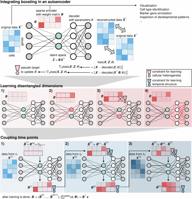
A BAE is an autoencoder with a specific architecture, where compL₂Boost is integrated into the gradient-based optimization scheme for the training. While the decoder of a BAE can be chosen arbitrarily, the encoder consists of only a linear layer

where B denotes the transposed encoder weight matrix. Note that extensions to more complex encoder architectures are possible, as discussed in “Discussion”.

Starting with a zero-initialized encoder weight matrix and randomly initialized decoder parameters, the optimization of the BAE in each training epoch is performed in an alternating manner by optimizing the encoder weights via successive application of the compL₂Boost algorithm to each latent dimension and optimization of the decoder parameters using a gradient-based optimization algorithm such as stochastic gradient descent or Adam. To integrate boosting as a supervised approach into an unsupervised optimization process, we define pseudo responses to update the linear model coefficients, corresponding to the rows of the encoder weight matrix.

Consider observations \({{{\boldsymbol{X}}}}\in {{\mathbb{R}}}^{n\times p}\) with standardized covariate vectors and a BAE with d ≪ p latent dimensions. Due to standardization, we work with normality assumptions and thus choose the mean squared error as the reconstruction loss:

In an arbitrary training epoch \(k\in {\mathbb{N}}\), let \({{{\boldsymbol{B}}}}=({{{{\boldsymbol{\beta }}}}}^{(1)},\ldots ,{{{{\boldsymbol{\beta }}}}}^{(d)})\in {{\mathbb{R}}}^{p\times d}\) denote the current transposed encoder weight matrix, where each column vector β^(l) represents the current regression coefficients and Z = (z⁽¹⁾, …, z^(d)) ≔ XB represents the latent representation, consisting of the current prediction vectors z^(l), for each latent dimension l = 1, …, d. The first step for updating the encoder weights is to compute the negative gradients of the training objective with respect to the prediction vectors z^(l) as pseudo responses, defining

The negative gradients represent the directions in which the predictions have to be adjusted to minimize the training objective the most. We standardize the pseudo responses to fulfill the required normality assumption for the compL₂Boost from “Componentwise likelihood-based boosting”, and to omit an intercept term

Note that after standardization, the pseudo responses still define descent directions for the training objective. Subsequently, updates for the regression coefficients, i.e., the weights of the encoder, are obtained via successively applying the compL₂Boost algorithm for only one boosting step with a step size ε ∈ (0, 1) to the pairs of observations and pseudo responses \({({{{{\boldsymbol{x}}}}}_{i},{\widehat{g}}_{i}^{(l)})}_{i = 1}^{n}\)

Subsequently, the decoder parameters are updated by performing one step of a gradient-based optimization scheme.

After training, the latent representation can be computed by feeding the data to the trained encoder f_enc, parameterized by the sparse encoder weight matrix. Each nonzero weight corresponds to a link between a latent dimension and one of the input variables. At the same time, its absolute value is an indicator of the importance of that variable.

Supplementary Algorithm 2 provides a pseudocode of the alternating core BAE optimization algorithm. We refer to this alternating optimization procedure as optimization in alternating mode. Although described in an alternating manner here, the gradients of the training objective w.r.t. z⁽¹⁾, …, z^(d) and the decoder parameters could be computed simultaneously on the same training batches. This would allow for parallelization of the subsequent update computations using different optimization criteria.

Alternatively, encoder and decoder can be trained jointly, which simplifies training by using an end-to-end instead of a two-step strategy, and allows for adding further layers to the encoder for capturing more complex patterns. This requires to differentiate through the boosting step in each epoch to obtain gradients of the reconstruction loss that respect the encoder parameter updates, which can be realized efficiently using differentiable programming⁸¹ and a flexible automatic differentiation framework⁵³ (see “Differentiable programming for joint optimization”).

Note that the activation functions need to be selected such that their derivatives do not vanish at zero, which happens, e.g., for standard implementations of the popular ReLU function. Otherwise the pseudo responses vanish and the encoder weight matrix stays zero during the entire training process.

Applying compL₂Boost for only one boosting step to each latent dimension results in a coarse approximation of the current pseudo responses in each training epoch, where only one element of the associated row vector of the encoder weight matrix is updated. However, applying the algorithm for only one step is sufficient, as the fit is carried out as part of an iterative optimization process.

In general, by training a BAE as described above, with d latent dimensions for a number of N training epochs, at least d elements but at most d ⋅ N elements of the encoder weight matrix become nonzero during the training. Consequently, the sparsity level of the encoder weight matrix is highly influenced by the number of training epochs and boosting steps. For reaching a desired sparsity level, we suggest limiting the maximum number of nonzero coefficients per dimension by training for a fixed number of epochs while adjusting the step size for the boosting component, regulating the number of nonzero coefficients. We believe that introducing regularization for the decoder parameters and the coefficients of the boosting component (see e.g., in refs. ^45,70) could further stabilize the variable selection when training for a large amount of epochs and prevent it from overfitting.

To illustrate the optimization process of the BAE and verify its effectiveness in representing distinct cell groups and identifying characteristic sparse gene sets in each latent dimension via modification of the selection criterion, we provide a simple simulation design in Supplementary Note 8 and a detailed analysis in Supplementary Note 9 and Supplementary Figs. 12 and 13. A comparison to potential alternative approaches using regularization techniques is provided in Supplementary Note 10 and Supplementary Figs. 14–19.

Disentanglement constraint for structuring latent representations

So far, we have explained the BAE optimization using unconstrained gradients as pseudo responses. To learn disentangled latent dimensions, we constrain the pseudo responses for the boosting in the encoder optimization. Consider the same setting as described in “Core optimization algorithm of the BAE for updating the encoder weight matrix”. For each latent dimension l = 1, …, d, instead of taking the standardized negative gradient \({\widehat{{{{\boldsymbol{g}}}}}}^{(l)}\) as the pseudo responses, only the fraction of the gradient that is currently not explainable by the other latent dimensions k ∈ {k = 1, …, d∣k ≠ l} is used as the constrained pseudo responses. Therefore, we first define by

the set of all indices of latent dimensions with corresponding all-zero encoder weights together with the current index l. Note that zero-weight vectors only occur in the first training epoch. The matrix \({{{{\boldsymbol{Z}}}}}^{(-{{{\mathcal{I}}}})}\) then consists of only the columns of Z whose indices do not appear in \({{{\mathcal{I}}}}\). The exclusion of zero columns is important for avoiding technical invertibility problems in the following computations. Next, we predict the best linear fit of \({{{{\boldsymbol{Z}}}}}^{(-{{{\mathcal{I}}}})}\) to the pseudo responses \({\widehat{{{{\boldsymbol{g}}}}}}^{(l)}\) by first computing the ordinary linear least squares estimator

and subsequently calculating the residual vector

The constrained pseudo responses for the boosting are then defined as the standardized vector

representing the fraction of the original pseudo responses \({\widehat{{{{\boldsymbol{g}}}}}}^{(l)}\) that is currently not explained by other latent dimensions k ∈ {k = 1, …, d∣k ≠ l}.

In the special case of updating β⁽¹⁾ during the first training epoch, where no variables have been selected yet, \({{{\mathcal{I}}}}=\{1,\ldots ,d\}\). In that case, we neglect the least squares estimation-step and directly set \({\widehat{{{{\boldsymbol{y}}}}}}^{(1)}={\widehat{{{{\boldsymbol{g}}}}}}^{(1)}\).

A pseudocode for the disentanglement constraint that can be included in the core optimization algorithm for adapting the pseudo response of each latent dimension in each training epoch is stated in Supplementary Algorithm 3.

Differentiable programming for joint optimization

For better communication between the encoder and decoder parameter updates, we provide an alternative optimization procedure for the BAE. While in the optimization process described in “Core optimization algorithm of the BAE” updates for the encoder- and decoder parameters are performed in an alternating way, they can also be optimized simultaneously using differentiable programming^52,53,81, a paradigm for flexibly coupling optimization of diverse model components. For an overview from a statistical perspective, see ref. ⁸². Specifically, we incorporate the boosting part of the optimization as part of a recursively defined joint objective L_joint(X; θ)

Hence, updates for the decoder parameters respect changes in the encoder parameters. Thereby, the θ subscript indicates the dependence on the current state of the decoder parameters. This procedure is facilitated by differentiable programming, which allows for jointly optimizing the neural network and boosting components by providing gradients of a joint loss function with respect to the parameters of all components via automatic differentiation. In particular, we use the Zygote.jl automatic differentiation framework⁵³, which allows for differentiating through almost arbitrary code without user refactoring.

By each call to the joint objective, when optimizing the decoder parameters in one training epoch via an iterative gradient-based optimization algorithm, boosting is performed in the forward pass, hence, the encoder weights are updated in the forward pass.

The joint version of the objective allows to adapt our alternating optimization algorithm to a stochastic framework, meaning that the joint objective can also be applied to randomly sampled mini-batches consisting of m ≤ n of the observation vectors. This enables the simultaneous optimization of the encoder and decoder parameters using the same mini-batch. Thus, the boosting part of the BAE optimization process acts on mini-batches, which is related to the stochastic gradient boosting approach described in ref. ⁸³.

Note that using the joint objective function for the optimization leads to a slight increase in training duration since the calculation of the reconstruction loss also incorporates the boosting step. Also, depending on the implementation of the mini-batch procedure, each training epoch could consist of updating all model parameters iteratively, using a partition of the whole dataset into distinct mini-batches of size m. Consequently, the boosting component could be applied several times per epoch, which affects the sparsity level of the encoder weight matrix.

We refer to this joint optimization procedure as optimization in jointLoss mode.

Adaptation for time series

As an additional use case, we illustrate an adaption of the BAE for handling time series data. Therefore, consider a T-tuple consisting of snapshots of observation data at different time points (X⁽¹⁾, …, X^(T)). E.g., these could be scRNA-seq datasets from the same tissue sequenced at different time points. The matrices might contain different numbers of observations/cells, i.e., \({{{{\boldsymbol{X}}}}}^{(i)}\in {{\mathbb{R}}}^{{n}_{t}\times p}\), for \({n}_{1},\ldots ,{n}_{T}\in {\mathbb{N}},t=1,\ldots ,T\).

We assume that the data reflects a developmental process of cells across measurement time points. For example, cells differentiate into different (sub-)types, and each process is characterized by a small gene set that gradually changes over time by sequential up- and downregulation of genes along the developmental trajectory. For each developmental process, we aim to capture the changes in the associated gene set in linked latent dimensions, one for each time point in an adapted version of the BAE, called timeBAE.

More precisely, the timeBAE comprises one BAE for each time point. The models are trained successively with the disentanglement constraint (see sections “Core optimization algorithm of the BAE” and “Disentanglement constraint for structuring latent representations”) for a fixed number of epochs on data from the corresponding time point using a pre-training strategy. At each time point, the encoder weight matrix from the previous time point is used for initializing the current encoder weight matrix. Once the complete training process is done, we concatenate all the encoder weight matrices and end up with a new stacked encoder weight matrix with d ⋅ N latent dimensions. For each k = 1, …, d, dimensions k + (t − 1)d for t = 1…T then represent the same developmental process across time. This requires some prior knowledge about the expected number \(d\in {\mathbb{N}}\) of developmental processes of cell groups.

For a formal description, consider T BAEs with linear encoders \({f}_{{{{\rm{enc}}}}}^{(T)}({{{\boldsymbol{x}}}};{{{{\boldsymbol{B}}}}}^{(T)}):= {({{{{\boldsymbol{B}}}}}^{(T)})}^{\top }{{{\boldsymbol{x}}}}\), where at the beginning of the training, \({{{{\boldsymbol{B}}}}}^{(0)}:= {{{{\boldsymbol{0}}}}}_{{{\mathbb{R}}}^{p\times d}}\). Each BAE is trained with the data from the respective time point. First, decoder parameters are initialized randomly. We denote the updated matrix obtained after training at time t by B^(t), and the next initialization of the encoder weight matrix at time t + 1 by \({\widetilde{{{{\boldsymbol{B}}}}}}^{(t+1)}\). We set \({\widetilde{{{{\boldsymbol{B}}}}}}^{(1)}:= {{{{\boldsymbol{B}}}}}^{(0)}\). Specifically, for the following time points we set

Thus, changes in previous encoder weights are incorporated as prior knowledge guiding the model to select genes corresponding to the same developmental program in the same dimension across time points. After training, the overall transposed encoder weight matrix is defined as \({{{\boldsymbol{B}}}}:= ({\widetilde{{{{\boldsymbol{B}}}}}}^{(2)},\ldots ,{\widetilde{{{{\boldsymbol{B}}}}}}^{(T+1)})\in {{\mathbb{R}}}^{p\times d\cdot T}\), and the joint encoder as f_enc(x; B) ≔ B^⊤x.

A reordered matrix B_perm, where the linked latent dimensions across time are grouped, can be constructed by reorganizing the columns of B as follows:

where \({\widetilde{{{{\boldsymbol{B}}}}}}_{(:,j)}^{(t)}\) represents the jth column of \({\widetilde{{{{\boldsymbol{B}}}}}}^{(t)}\), for t ∈ {2, …, T + 1} and j ∈ {1, …, d}.

Note that this approach is compatible with both training in alternating and in jointLoss mode.

Determining correspondence of latent patterns to cell types

In situations where cell labels of k categories, such as cell types, are already available, the learned patterns in different BAE latent dimensions can be checked for overlap with the label patterns. For this purpose, a quantile thresholding strategy is used to check the top positive and negative representation values of each latent dimension for overlap with the cell type patterns. Let \({{{\boldsymbol{Z}}}}\in {{\mathbb{R}}}^{n\times d}\) represent the d-dimensional BAE latent representation of n cells. For j = 1, …, d we first compute the p ∈ (0, 1) quantile \({q}_{+}^{(j)}\) and the (1 − p) quantile \({q}_{-}^{(j)}\) given the representation vector z^(j) in dimension j. Next, we determine the indices of cells with a representation value above \({q}_{+}^{(j)}\) and check the different label proportions \({p}_{+,l}^{(j)}\in [0,1],l=1,\ldots ,k\), e.g., cell type proportions, and do the same for cells with a representation value below \({q}_{-}^{(j)}\). The label that best matches the learned positive patterns in the latent dimension j is

The label that best matches the learned negative patterns can be computed in a similar way. For the BAE analysis on the cortical mouse data, we set p = 0.9.

Identification of top selected genes per latent dimension

In contrast to standard iterative gradient-based parameter optimization, which starts from a random initialization of the parameters, we presented an optimization approach that starts from a zero initialization and allows the iterative selection of the parameters to be updated. Iteratively updating the BAE encoder weights using componentwise boosting results in a sparse encoder weight matrix where many of the weights are truly zero. However, the nonzero weights in the encoder weight matrix link variables, i.e., genes, with different latent dimensions, and the magnitude of their values reflects the effect on the representation in the dimensions. Taken together, the two most important pieces of information that can be derived from the encoder weight matrix are (1) knowledge of which genes have been selected (nonzero weights), and (2) how strongly the genes are associated with the latent dimensions. The latter is especially important when training for a large number of training epochs, where weights are selected and updated in a forward selection manner. To identify the top genes, i.e., the most influential genes for the different latent dimensions, we suggest examining per individual latent dimension, the scatter plots of the encoder weights sorted in descending order by their absolute value. In addition, a change-point criterion can be used to identify the genes with a nonzero weight per latent dimension that have the greatest influence on the representation. The change-point genes for a latent dimension can be identified by first sorting the nonzero absolute values of the corresponding encoder weights in descending order. Then, pairwise differences are computed for the neighboring elements in the sorted vector. The maximum value of the differences indicates where the change point is, i.e., where the order of magnitude of the absolute values of the weights decreases the most. For example, if the maximum value of the differences is the third element, then the first three genes are considered to be the change-point genes, i.e., the top genes.

Label predictions of unseen data

Given that the cells used to train the model are labeled, label predictions for unseen cells can be performed. First, the unseen cells are mapped to the latent space using the trained encoder of the BAE. Labels for these cells are then predicted by identifying the k nearest neighbors in the low-dimensional latent space, using a distance metric such as Euclidean distance. The most frequent cell type among these k neighbors is assigned as the predicted label for each unseen cell. For the analysis of the cortical mouse data in “The BAE identifies cell types and corresponding marker genes in cortical neurons”, we set k = 10.

Gene selection stability analysis

To investigate the robustness in terms of gene selection stability on the cortical mouse data, we repeatedly trained a BAE under the same training conditions as described in “Statistics and reproducibility”, but using different initializations for the decoder parameters. We determined the number of times each gene was selected across 30 runs. For each run, we examined whether the weights corresponding to the gene in at least one latent dimension were nonzero. If so, the gene was considered selected for that run, contributing a count of 1. The total selection count for each gene was then calculated as the sum of its selections across all 30 runs.

Robustness analysis of structuring latent representations

The robustness of the BAE was assessed in its ability to learn well-structured latent representations under more challenging conditions, such as increased noise levels or weaker signals. To achieve this, we leveraged the gene selection stability analysis results for the BAE (see “Gene selection stability analysis”, Supplementary Note 4, Supplementary Fig. 6, and Supplementary Table 3) and systematically replaced the top q% of the most frequently selected genes in the cortical mouse dataset (1525 cells and 1500 highly variable genes) with noise genes. Noise genes were defined as randomly selected genes that were expressed in at least one cell and distinct from the set of 1500 highly variable genes. We trained the BAE under the same training conditions outlined in “Statistics and reproducibility“ for different percentages q and visually compared the outcomes. The results are presented in Supplementary Note 5, Supplementary Fig. 7, and Supplementary Table 4.

Clustering analysis of BAE and PCA based representations of cortical neurons

We trained a BAE with 10 latent dimensions using 20 different decoder parameter initializations in alternating mode with the disentanglement constraint on cortical neurons stemming from the primary visual cortex of mice. After training, we computed the corresponding 20 latent representations of the data. On the other hand, we computed the PCA representation of the data where we only kept the first ten principal components equaling the number of latent dimensions of the BAE. Since PCA is a deterministic approach, we performed Leiden clustering for 20 seeds, resulting in 20 different PCA clusterings. In contrast, we performed Leiden clustering once for each BAE representation.

Subsequently, we evaluated and compared the clustering results using two popular metrics for cluster analysis, the silhouette score and the adjusted Rand index (e.g., see refs. ^84,85,86). The silhouette score is a general quality measure for a single clustering, which is defined as the mean of silhouette coefficients of the clustering. For each observation, the corresponding silhouette coefficient measures how well the observation fits into its cluster compared to others. The silhouette coefficient takes values in [−1, 1]. A value of one corresponds to an observation fitting well to its assigned cluster compared to other clusters, and a value of −1 means that the observation fits better to other clusters compared to its own. The adjusted Rand index is a version of the Rand index that is corrected for random chance measuring the similarity of two clusterings. A value of one means that both clusterings are identical, whereas a value of zero corresponds to random labeling. We used the scikit-learn implementation for both clustering metrics.

We report the median silhouette score of the 20 clusterings for each method together with the interquartile ranges of silhouette scores, as well as the median adjusted Rand index, for quantitatively comparing the clustering results (see “The BAE identifies cell types and corresponding marker genes in cortical neurons”).

Model comparison for gene selection

We compared the BAE to two other sparse unsupervised variable selection approaches for gene selection: (1) sparsePCA⁴⁰ and (2) single-cell Projective Non-negative Matrix Factorization (scPNMF)⁶⁵. Like the BAE, both approaches aim to establish sparse connections from the gene space to different dimensions in a low-dimensional space. Brief descriptions of these methods are given below and detailed explanations are available in the respective references^40,65.

sparsePCA

sparsePCA⁴⁰ is a modification of the original PCA formulation that additionally constrains the resulting loading matrix to be sparse. Let \({{{\boldsymbol{X}}}}\in {{\mathbb{R}}}^{n\times p}\) denote the data matrix with n observations, e.g., cells and p variables, e.g., genes. The optimization problem solved can be formulated as a PCA problem (dictionary learning⁸⁷) with an ℓ₁ penalty on the \(d\in {\mathbb{N}}\) components:

where ∥ ⋅ ∥_F denotes the Frobenius norm, ∥ ⋅ ∥₂ is the Euclidean norm, and ∥ ⋅ ∥₁ is the sum of the absolute values of all matrix entries. The sparsity level can be adjusted through the hyperparameter α. Increased values of α lead to an increased sparsity level of the resulting loading matrix \({{{\boldsymbol{V}}}}\in {{\mathbb{R}}}^{d\times p}\). For our analysis, we used the scikit-learn (v1.4.0) implementation of sparsePCA which is based on ref. ⁸⁷.

scPNMF

scPNMF⁶⁵ is an extension of the Projected Non-negative Matrix Factorization (PNMF) algorithm^88,89 that is constrained to learn a sparse loading matrix consisting of only positive elements, specifically tailored for scRNA-seq data analysis.

The algorithm takes as input a log-transformed count matrix \({{{\boldsymbol{X}}}}\in {{\mathbb{R}}}_{\ge 0}^{n\times p}\), with n cells and p genes. Given a number of dimensions \(d\in {\mathbb{N}}\), the goal of PNMF is to identify a representation of the data in a d-dimensional space in which the dimensions are defined as nonnegative, sparse, and mutually exclusive linear combinations of the p genes⁶⁵. To achieve this, PNMF solves the following optimization problem:

Here, W is a matrix whose entries are in addition constrained to be nonnegative. The optimization problem is initialized with a nonnegative loading matrix and solved using an iterative optimization algorithm⁶⁵. During each update iteration, elements in W that fall below a specified threshold are set to zero.

A second important step in the scPNMF workflow is post-hoc basis selection of the resulting loading matrix, where dimensions are filtered whose corresponding components do not reflect a biological pattern or are correlated with cell library sizes⁶⁵. However, since post-hoc basis selection could in principle be performed also for the BAE, we excluded it from our comparison and concentrate on the comparison of the outputted loading matrix, i.e., encoder weight matrix.

For the model comparison, we used the same dataset for both the BAE and sparsePCA, comprising 1,525 neural cells from the cortical mouse data. The data was standardized prior to parameter optimization, as detailed in “Data preprocessing”. For scPNMF, log-transformed normalized count values with a pseudo-count of one were used instead. All approaches were restricted to selecting genes from the set of the 1500 most highly variable genes. We ran sparsePCA and scPNMF with their default hyperparameter settings, but set the number of components, i.e., latent dimensions, to 10. The approaches were compared in terms of gene selection, specifically the sparsity of the sparsePCA and scPNMF loading matrices and the BAE encoder weight matrix. Consistent with the gene selection stability analysis (see “Gene selection stability analysis”), we trained the BAE 30 times under identical training conditions but with different initializations of the decoder parameters. Similarly, sparsePCA and scPNMF were run 30 times with varying seed parameters. A gene was considered selected in a run if it had at least one nonzero element across the 10 components in the resulting BAE encoder weight matrix or loading matrices. The results are presented in Supplementary Note 6 and Supplementary Table 5.

Simulation of scRNA-seq-like data with time structure

To simulate scRNA-seq-like data with time structure representing a developmental process of three different cell groups across three time points, we followed the simulation design presented in ref. ³⁵ (see also Supplementary Note 8, Supplementary Fig. 12, and Supplementary Table 7). We generated one binary count matrix for every time point representing a snapshot of the current state of the three cell groups. To enable a more realistic scenario, the data at each time point consists of a different number of cells and p = 80 genes. Specifically, a cell taking the value 1 for some gene indicates a gene expression level exceeding a certain threshold for that cell, whereas the value 0 indicates an expression level below that threshold. The data at each time point is modeled by i.i.d. random variables \({({X}_{i,j} \sim {\mbox{Ber}}({p}_{i,j}))}_{i = 1,\ldots ,n,j = 1,\ldots ,p}\), where p_i,j denotes the probability of a value of 1 for a gene j in a cell i. We set p_i,j to 0.6 for highly expressed genes (HEGs) and to 0.1 for lowly expressed genes (LEGs). To model a smooth transition between two successive cell stages across subsequent time points, we include overlaps between the sets of HEGs from two subsequent time points. Table 1 comprises the details of the gene expression patterns and overlap patterns for the count matrices at different time points. In total there are 54 HEGs for the different cell stages and 26 genes that are lowly expressed in all cell stages across all time points that are added as non-informative genes to make the variable selection task more challenging and realistic. For simplicity, we strictly excluded intersections between the sets of HEGs of distinct cell groups. An exemplary visualization of simulated time series scRNA-seq data can be found in Fig. 4a.

Gene selection comparison for the timeBAE

In a setting where both temporal information and cluster identities are available, we can compare the sets of selected genes of the timeBAE to the ones obtained by fitting linear models given the cluster and time point information. The process involves the following steps:

The trimmed embryoid body dataset is first divided into subsets corresponding to different time points (X⁽¹⁾, …, X^(T)) in the same way as for training the timeBAE. Next, for each time point t and cluster c, binary response variables are defined as follows:

leading to response vectors:

where n_t is the number of cells measured at time t, and t ∈ {1, …, T},  c ∈ {1, …, C}. We fit multivariate linear regression models without intercept terms using standardized predictors and responses at each time point:

Despite the binary nature of the response, linear models are employed to focus on identifying significant coefficients representing characteristic genes rather than predictive accuracy. To identify the genes most characteristic of a cluster at a given time point, we test for each coefficient if it significantly differs from zero via a two-sided t-test. P-values are adjusted for multiple testing using the Bonferroni correction for each fitted regression model. Only genes corresponding to coefficients that were significantly different from zero were counted as selected (coefficients with adjusted p-values below the significance level α = 0.05).

Inspecting the UMAP plots colored by the timeBAE latent dimensions, each set of linked timeBAE latent dimensions is visually assigned to the corresponding cluster. For each set of linked latent dimensions, we next compute the intersection of the selected genes for each latent dimension and the set of genes selected by the corresponding linear model. The results are reported in Supplementary Table 6.

Statistics and reproducibility

All code to run the model and reproduce all analysis results and figures is publicly available at https://github.com/NiklasBrunn/BoostingAutoencoder, including documentation and a tutorial in a Jupyter notebook using the Julia programming language, illustrating the functionality of the approach in a simulation study (see Supplementary Note 8, Supplementary Table 7, and Supplementary Fig. 12).

The BAE and its modification for analyzing time series data are implemented in the Julia programming language⁹⁰, v1.6.7, using the packages BenchmarkTools (v1.5.0), CSV (v0.10.11), Clustering (v0.15.7), ColorSchemes (v3.24.0), DataFrames (v1.3.5), Distances (v0.10.11), Distributions (v0.25.100), Flux (v0.12.1), GZip (v0.5.2), MultivariateStats (v0.10.3), Plots (v1.24.3), ProgressMeter (v1.9.0), StatsBase (v0.33.21), UMAP (v0.1.10), VegaLite (v2.6.0), XLSX (v0.10.0). Scripts for downloading and preprocessing the embryoid body data and parts of the preprocessing of the cortical mouse data are implemented in Python v3.10.11. We added a YAML file to our GitHub repository containing the information about the used packages and corresponding versions. Users can create a conda environment for running the Python code from the YAML file.

In all our experiments, the encoder of any BAE is defined by

where the matrix \({{{\boldsymbol{B}}}}\in {{\mathbb{R}}}^{p\times d}\) denotes the transposed encoder weight matrix and we used 2-layered decoders

where \({{{{\boldsymbol{W}}}}}^{(1)}\in {{\mathbb{R}}}^{p\times d},{{{{\boldsymbol{b}}}}}^{(1)}\in {{\mathbb{R}}}^{p},{{{{\boldsymbol{W}}}}}^{(2)}\in {{\mathbb{R}}}^{p\times p}\) and \({{{{\boldsymbol{b}}}}}^{(2)}\in {{\mathbb{R}}}^{p}\) denote the trainable weight matrices and bias vectors.

The number of units in the input and output layers corresponds to the number of variables in the datasets (i.e., p = 1500 for the cortical mouse data analysis and subgroup analysis, p = 80 in the time series simulation, p = 263 on the embryoid body dataset, and p = 50 in the stair-like simulation design from Supplementary Note 8). The number of latent dimensions was selected according to a rough estimate of the number of groups present or expected in the datasets. Specifically, we used d = 10 latent dimensions for the cortical mouse data comprising cells of 15 neuron cell types, d = 4 for the subgroup analysis of Sst-neurons, d = 3 in the time series simulation where we simulated three groups of developing cells, d = 4 for the embryoid body data where we obtained three clusters from Leiden clustering with a resolution parameter of 0.025, and d = 10 in the stair-like simulation design where we simulated ten groups of cells.

In the boosting part of the optimization, we set the number of boosting steps to M = 1 and the step size to ε = 0.01 for all experiments. Specifically, we applied BAEs using the disentanglement constraint in alternating mode to obtain the presented results for the embryoid body data, the clustering analysis on cortical mouse data and the stair-like simulation design, and in jointLoss mode for obtaining the results for the remaining datasets. We chose m = 500 as the common batchsize for optimizing encoder and decoder parameters for the cortical mouse data, m = 95 for application on the Sst-neurons, m = 198 for the simulated time series scRNA-seq data, m = 1500 as the batchsize for decoder parameter optimization for the embryoid body data, and m = 800 as the batchsize for decoder parameter optimization for the stair-like simulation design. In every scenario, we used the Adam optimizer⁶² for updating the decoder parameters, where the learning rate was set to ν = 0.01. The number of training epochs was set to 25 for obtaining the here presented results on the cortical mouse data, 20 for the Sst-neurons, 9 for training the timeBAE with data at each time point of the simulated scRNA-seq data, 15 for training with data at each time point of the embryoid body data, and 15 for the stair-like simulation design.

Computation time and memory

A key focus in the present manuscript is the applicability of the BAE to small data scenarios, e.g., for helping to identify and characterize rare cell types. We have thus not specifically investigated on scalability in the current implementation. In Table 2, we present the computation time and total allocated memory for the optimization process in the main experiments. All experiments were conducted on a MacBook Pro (2023) with an Apple M2 Max chip (12-core CPU, 38-core GPU) and 96 GB of RAM. The required computation times and memory were measured using the @btime macro from Julia’s BenchmarkTools package. The reported times and memory represent the minimum execution time and total allocated memory across multiple runs, ensuring robust performance evaluation by minimizing noise.

Data preprocessing

For the adult mouse cortical scRNA-seq data⁶¹, we downloaded the expression data consisting of the measured gene expression levels of 15,119 genes in 1679 single cells, the gene names, and cell type annotations from GEO under accession number GSE71585. Next we removed the samples which have been flagged by Tasic et al.⁶¹ as being of bad quality. As the quantification of aligned reads per gene has been conducted with RSEM⁹¹, decimal numbers might show up occasionally in the estimated counts per gene. Next, we normalized the data using the DESeq2 normalization for sequencing depth⁹² to adjust for fluctuations in the number of aligned reads per sample, affecting each gene’s estimated expression level. Afterward, we log-transformed the normalized counts with an added pseudo-count of one. Genes were removed if count values did not exceed ten in more than 20 cells. Our analysis focused on the subset of cortical neurons based on the cell type annotation provided by Tasic et al.⁶¹. We removed genes expressed in less than ten cells for the remaining cells. Further, we reduced the set of genes to 1500 highly variable genes using the built-in scanpy (v1.9.8) function for highly variable gene selection with the flavor variable set to ‘seurat’, including marker genes of neural cell types (Fig. 3 and Supplementary Fig. 12 in ref. ⁶¹) and neurotransmitter receptor genes (Supplementary Fig. 15 in ref. ⁶¹) that were previously identified in ref. ⁶¹ (Fig. 3 in ref. ⁶¹). The resulting count matrix consists of 1525 neurons and 1500 highly variable genes, including 90 of the 180 neural marker and receptor genes identified by Tasic et al.⁶¹.

In the subgroup analysis of cells highly expressing the marker Sst, we first selected only the Sst-neurons. Subsequently, we removed genes expressed in less than ten cells, followed by highly variable gene selection using the built-in scanpy (v1.9.8) function for highly variable gene selection with the flavor variable set to “seurat”. The resulting count matrix consists of 202 Sst-neurons with gene counts of 1500 highly variable genes.

The embryoid body data comprises gene expression levels of embryonic cells generated over a 27 day time course, stored in five different count matrices depending on measurement time. Especially, cells sequenced at days 0–3 were labeled as time point 1, cells from day 6 to 9 as time point 2, cells from day 12 to 15 as time point 3, cells from day 18 to 21 as time point 4, and cells from day 24 to 27 as time point 5. We excluded cells from time point 1 since their expression patterns are mostly homogeneous. For the remaining cells, we followed and adapted the preprocessing steps from ref. ⁶⁶. First, we filtered cells by library size to remove doublets and empty droplets, where for each time point cells below the lower 20th percentile and above the upper 20th percentile were excluded. Next, we filtered genes expressed in less than ten cells, separately for each time point. We further excluded apoptotic cells expressing a large total amount of mitochondrial genes The threshold was set to 400. Subsequently, we normalized the counts for each cell by dividing each count value by the total number of counts across genes. Next, we re-scaled the normalized counts by a factor of 10,000, followed by a log-transformation with a pseudo-count of one. For the timeBAE analysis, we fused the data matrices from time points 3 and 4, creating the new time point 34 for those cells, and subset the data to cells that can be grouped in large clusters. Therefore, we performed PCA and chose the first 50 principal components to apply the Leiden clustering algorithm with resolution parameters of 0.025 and 0.25. Under observation of the clustering results with the resolution parameter 0.25 in a 2D UMAP plot of cells, we then removed clusters that were separated from the larger groups. Next, we selected genes that were differentially expressed between different clusters of the clustering with resolution parameter 0.025 using the built-in scanpy (v1.9.8) function for differentially expressed gene detection with the method variable set to “wilcoxon”. In addition, we selected genes differentially expressed between the adapted time points for each individual cluster. After preprocessing and filtering, we ended up with 11,627 cells and a combined set of 262 differentially expressed genes.

Since the BAE approach requires observation data in a standardized form, z-scores of the gene vectors were computed for each of the simulated and real-world scRNA-seq datasets. We used the log-transformed counts to standardize the mouse cortical scRNA-seq data and the embryoid body scRNA-seq data. For the simulated scRNA-seq datasets, we re-scaled the noise variables after standardization by multiplying them with a scalar factor to adjust the range of the values to that of the other gene vectors. The scaling factor for the simulated scRNA-seq data with time structure was set to 0.5, and for the stair-like scRNA-seq data for the analysis of the BAE functionality in Supplementary Note 9 to \(\frac{2}{3}\).

All scripts for loading and preprocessing the different datasets are available in our GitHub repository https://github.com/NiklasBrunn/BoostingAutoencoder.

Reporting summary

Further information on research design is available in the Nature Portfolio Reporting Summary linked to this article.