Identifying and forecasting importation and asymptomatic spreaders of multi-drug resistant organisms in hospital settings

Dataset

We extract three different types of patient data based on the electronic health records (EHR) from the University of Virginia hospital: patient demographic information and risk factors (e.g., comorbidities, medical history), lab testing, and contact network data.

• Patient risk factor data: This dataset consists of risk factors for all patients in ICUs. From the EHR dataset, we collected 19 different risk factors for each patient, all of which are available before ICU admission. From July 1, 2019, to December 31, 2019, there were 1117 patients in UVA ICUs, and 74 of them were MRSA importation cases (all patients received an MRSA test within (t − 3, t + 3) days of being admitted into one of the ICUs, and patients who tested positive for MRSA within this range are considered as importation cases). A list and description of each risk factor are provided in the Supplementary Information.

• Lab testing data: This dataset consists of infection data for each patient. There were two different types of tests to diagnose MRSA: culture tests and polymerase chain reaction (PCR) tests. However, since a negative culture test cannot disqualify an individual from MRSA infection, we focused on only positive culture tests and both positive and negative PCR tests. For a given patient p on a given day t, y_p,t = 1 represents that the patient was tested positive on day t or if their most recent test in the past was positive. Likewise, y_p,t = 0 if this patient was tested negative on day t or if their most recent test was negative.

• Contact network data: This dataset consists of a series of ward-level co-location contact networks A_t comprising three different entities: patients, healthcare workers (HCWs), and locations, and each network is for one specific day. From the EHR dataset, we can collect the movement information of patients and HCWs (e.g., the ward that a patient stayed, and when the doctors and nurses visited a specific ward). Note that these movement information also includes start and end times; we can infer whether these patients and HCWs were co-located (i.e., time overlapped) at any specific location. Specifically, if two patients or HCWs v₁, v₂ colocated at location l on day t, we would create edges between v₁ and v₂, v₁ and l, v₂ and l on day t in A_t. However, because of the nature of this data, individuals such as support staff or patient guests are not tracked, and thus are not included in the network. Additionally, HCW-HCW colocations are not tracked in rooms where care is not administered, such as break rooms. From July 1, 2019 to December 31, 2019, there were 1117 patients (and 6445 patient days), 2385 healthcare workers, and 77 locations in the UVA ICU.

Problem setup

We use the trained NeurABM model to identify importation and nosocomial infection cases. For importation cases, the patient-specific parameter θ_p in this work is importation probability for each patient. Specifically, for each week k, we used the contact networks, patient risk factors, and lab testing results until week k to train the NeurABM, and our task is to identify the importation cases from them until week k. Note that NeurABM framework do not access to the ground-truth importation cases data. Instead, we only use the ground-truth importation cases data for evaluation.

For identifying current nosocomial infection cases in hospital, we follow the setup of a previous work²²: In this setup, since we want to identify current nosocomial infections in week k, we should be exactly in week k (e.g., at the end of week k). Therefore, for each week k, we used the contact networks, patient risk factors, and lab testing results until week k − 1 to train the NeurABM, and then ran the SIS-ABM model for 7 more days to infer the infection states of all patients for week k. Since we are identifying current nosocomial infection cases in week k, the contact network in week k is known, while the lab test results are not fully available (because of the delays in getting the lab test results). For example, if we were at the end of week 40 (beginning of October), we would train NeurABM on all the data from week 28 (beginning of July) to week 39. As for week 40, we would only use the contact network in that week and use the ABM simulator to identify the nosocomial infection cases in week 40. Then, at the end of week 41, we would train on the data from week 29 to 40 and identify the nosocomial infection cases in week 41. We repeated this procedure until we were at the end of week 52.

For forecasting future nosocomial infection cases, we followed a real-world step-forward scenario that made weekly predictions. In this setup, since we want to forecast future nosocomial infection cases in week k, we should be before week k (e.g., at the end of week k − 1). Therefore, for each week k, we used the contact networks, patient risk factors, and lab testing results until week k − 1 to train the NeurABM, and then ran the SIS-ABM model for 7 more days to forecast the infection states of all patients for week k without knowing any information for week k. For example, if we were at the end of week 39, we would train on the data from week 28 to week 39 to forecast for week 40 (i.e., no information from week 40 is used). Then, at the end of week 40, we would train on the data from week 29 to 40 and forecast for week 41. We repeated this procedure until we were at the end of week 52. Intuitively, the key difference between the setup of identifying current nosocomial infection cases and forecasting future nosocomial infection cases is whether the contact network in the targeted week k is known or not.

Transmission model

In this work, we use the SIS-ABM model in NeurABM to capture the MRSA spread dynamics in UVA ICUs³⁹. SIS-ABM is a pathogen load-based model that keeps track of pathogen load on all people and locations using a load vector l_t. For each patient i, they can either be in the Susceptible (S) or Carriage (C) state. Specifically, the probability of transitioning from S to C is proportional to the amount of pathogen on this patient l_t(i), which can be formulated as a linear dose-response function βl_t(i) (β is the disease infectivity parameter). Once in the carriage state, the patient keeps shedding more pathogen loads at each step, which can later be transferred to its neighbors (including both people and locations). Such a shedding process continues until the patient recovers with a recovery probability δ.

For the pathogen load transfer, as described in the previous text, the SIS-ABM model uses daily contact networks A_t to capture the exchange of pathogens among patients, HCWs, and locations. Specifically, we construct a transfer matrix R_t for each day t, where R_ijt = τ_ijtA_ijt. Here, A_t is the adjacency matrix of contact networks on day t, and τ_ijt is the transfer ratio parameter (the ratio of pathogen being transferred (or remaining if i = j) from patient/HCW/location j to patient/HCW/location i on day t). Specifically, based on the kinds of nodes of i and j, we have 8 kinds of transfer ratios: τ_PP, τ_PH, τ_PL, τ_HP, τ_HH, τ_HL, τ_LP, τ_LH. It also uses γ_P, γ_H, γ_L to denote the natural pathogen reduction rate on patient, HCW, and location nodes. Using this R_t and l_t(i), the SIS-ABM model updates the pathogen loads every day as a linear operation. We also restrict the column-sums of R_t to be less than or equal to 1, which implies that the total amount of pathogen cannot increase after transfer (i.e., ∣R_tl_t∣ ≤ ∣l_t∣). Note that susceptible patients may still carry a small amount of pathogen loads and spread them to others, and HCWs and locations are always in the susceptible state, which means that they can spread the MRSA pathogen loads but are non-infectable. We provide more details in the Supplementary Information.

NeurABM framework

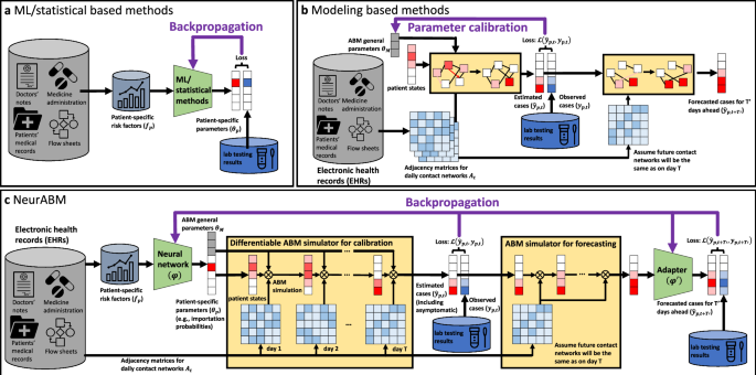
As shown in Fig. 1, the NeurABM framework is composed of two parts: the neural network part (green block, parameterized by ϕ) and the agent-based model simulator part (yellow blocks).

For the neural network component, we take the risk factors f (where f_p is for patient p) as input and then estimate both the patient-specific parameters θ_p (which is a vector and each element θ_p is for patient p and only influenced by the patient itself’s risk factors f_p, in this work it is importation probability for each patient) and ABM parameters θ_M (i.e., the general parameters that apply to every patient in the SIS-ABM model, including disease infectivity parameter β, recovery probability δ, pathogen shedding rate α, natural pathogen reduction rate for patients, HCWs, and locations γ_P, γ_H, γ_L, transfer ratios from different kinds of nodes τ_PP, τ_PH, τ_PL, τ_HP, τ_HH, τ_HL, τ_LP, τ_LH) together. The neural network is parameterized by ϕ and we use θ_p, θ_M = NN(f; ϕ) to represent it. We list all ABM parameters in Supplementary Information.

For the ABM simulator, we implement the simulation process of the SIS-ABM model using matrix operations in a differentiable way. ABM simulator takes the adjacency matrices of contact networks A_t and the parameters learned by neural networks (θ_p, θ_M) as input, and simulates MRSA spread in T days to estimate patient states on each day \({\hat{\boldsymbol{y}}}\) (where \({\hat{y}}_{p,t}\) is for patient p on day t). Specifically, the simulation process of the SIS-ABM model can be decomposed into three substeps: (1) pathogen load transmission where the load transfers via contact edges, (2) updating the states for each patient based on their pathogen loads and recovery probability, and (3) updating the timestep from day t to day t + 1. This process can be repeated for arbitrary steps to simulate the MRSA spread over T days. We use \({\hat{\boldsymbol{y}}}=ABM({\boldsymbol{A}};{{\boldsymbol{\theta }}}_{p},{{\boldsymbol{\theta }}}_{M})\) to represent it.

We also have another ABM simulator for forecasting. Since we cannot exactly know future contact networks, we assume they will be the same as the contact network on day T (i.e., A_T). Therefore, it takes the patient states on day T as the input and forecast for \(T^{\prime}\) days ahead. It can be represented by \(\hat{\boldsymbol{y}}_{F}^{\prime} =AB{M}_{F}({\hat{\boldsymbol{y}}};{{\boldsymbol{A}}}_{T},{{\boldsymbol{\theta }}}_{p},{{\boldsymbol{\theta }}}_{M})\). However, the assumption on the future contact networks is inaccurate and lead to bias in \(\hat{\boldsymbol{y}}_{F}^{\prime}\) we forecast. Therefore, we use another adapter neural network \(\phi^{\prime}\) to revise \({\hat{\boldsymbol{y}}}^{\prime}_{F}\) and give our final forecast \({\hat{{\boldsymbol{y}}}}_{F}\). We formulate it as \({\hat{{\boldsymbol{y}}}}_{F}=Adapter(\hat{\boldsymbol{y}}_{F}^{\prime} ,{\boldsymbol{f}};\phi^{\prime} )\).

With the aforementioned neural network and the ABM simulator, we then integrate them together to train simultaneously. Specifically, one training epoch comprises the following steps.

• Step 1: We feed the risk factor data f into the neural network as the input to estimate the patient-specific parameters θ_p. In this work, θ_p is the probability of being importation cases for each patient p. It is a vector of size N, where N is the number of patients in the contact network. Meanwhile, the neural network will also give the general ABM parameters θ_M that are applied to all patients (e.g., β, α, ⋯ ).

• Step 2: We then feed θ_p, θ_M, and the contact networks A_t into the ABM simulator and simulate for T steps. The output will be the vector \(\hat{{\boldsymbol{y}}}\) of size N × T, in which \({\hat{y}}_{p,t}\) represents the probability of being in the state carriage for patient p on day t.

• Step 3: We compare the estimated carriage probability \(\hat{{\boldsymbol{y}}}\) with the corresponding ground-truth observations (i.e., known carriage patients based on lab testing) y. We use the weighted binary cross entropy loss (BCE loss)⁴²\({\mathscr{L}}(\hat{{\boldsymbol{y}}},{\boldsymbol{y}})={\sum }_{p}{\sum }_{t}{w}_{pos}{y}_{p,t}\log ({\hat{y}}_{p,t})+{w}_{neg}(1-{y}_{p,t})\log (1-{\hat{y}}_{p,t})\) as the loss function. Here w_pos and w_neg are the weights for positive and negative observations. We set \({w}_{pos}:{w}_{neg}={\sum }_{p}{\sum }_{t}{\mathbb{1}}[{y}_{p,t}=0]:{\sum }_{p}{\sum }_{t}{\mathbb{1}}[{y}_{p,t}=1]\), where \({\mathbb{1}}[\cdot ]\) is the indicator function, which is 1 if the condition is true, and 0 otherwise.

• Step 4: Meanwhile, we also feed the \({\hat{y}}_{p,t}\) for day T to another ABM simulator to forecast for \(T^{\prime}\) days ahead. Note that these \(T^{\prime}\) days are for future and we cannot access to the real contact networks when forecasting, we assume that future contact networks will be the same as what we have for day T. Let ABM_F be this ABM simulator for forecasting, and \({\hat{\boldsymbol{y}}}^{\prime}_{F}\) of size \(N\times T^{\prime}\) as rough forecast output (in which \(\hat{y}^{\prime}_{p,t+T^{\prime}}\) represent the probability of being in the state carriage for patient p on day \(t+T^{\prime}\)), we formulate it as \({\hat{\boldsymbol{y}}}^{\prime}_{F} =AB{M}_{F}({\hat{\boldsymbol{y}}};{{\boldsymbol{A}}}_{T},{{\boldsymbol{\theta }}}_{p},{{\boldsymbol{\theta }}}_{M})\).

• Step 5: However, the assumption that future contact networks will be the same as on day T is inaccurate and leads to bias in \(\hat{y}^{\prime}_{p,t+T^{\prime}}\). To tackle this, we use another adapter neural network \(\phi^{\prime}\) to revise this rough output to get the revised forecast output \({\hat{{\boldsymbol{y}}}}_{F}\) of size \(N\times T^{\prime}\), in which \({\hat{y}}_{p,t+T^{\prime} }\) represents the probability of being in the state carriage for patient p on day \(t+T^{\prime}\). We formulate it as \({\hat{{\boldsymbol{y}}}}_{F}=Adapter({\hat{\boldsymbol{y}}}^{\prime}_{F} ,{\boldsymbol{f}};\phi^{\prime} )\) and compute the BCE loss \({\mathscr{L}}({\hat{{\boldsymbol{y}}}}_{F},{{\boldsymbol{y}}}_{F})={\sum }_{p}{\sum }_{t}{w}_{pos}{y}_{p,t+T^{\prime} }\log ({\hat{y}}_{p,t+T^{\prime} })+{w}_{neg}(1-{y}_{p,t+T^{\prime} })\log (1-{\hat{y}}_{p,t+T^{\prime} })\).

• Step 6: With the total loss \({\mathscr{L}}(\hat{{\boldsymbol{y}}},{\boldsymbol{y}})\) + \({\mathscr{L}}({\hat{{\boldsymbol{y}}}}_{F},{{\boldsymbol{y}}}_{F})\), and the differentiable ABM simulator, we can calculate the gradient of the loss with respect to the neural network parameters ϕ and adapter parameters \(\phi^{\prime}\) via backpropagation. This allows us to better tune the neural network and learn more reasonable parameters as the input for the ABM simulator.

The above steps are repeated until the total loss converges. Sometimes, directing the whole NeurABM framework can be extremely hard, since the framework can be really deep. Intuitively, if we use T days for ABM calibration and forecast for T′ days ahead, the depth of the framework becomes at least T+T′. To address this problem, an iterative training approach following previous work can be helpful: We can iteratively freeze different parts of the frameworks and train the other parts, allowing us to simplify the training NeurABM by breaking it down into two substeps: (1) First, we focus on training the neural network and the ABM simulator while keeping the adapter and ABM simulator for forecasting frozen, which allows us to first learn reasonable ABM parameters. (2) We then focus on the adapter and the ABM simulator for forecasting while keeping others frozen, which allows us to learn reasonable parameter for adapter. These two substeps above can be repeated until convergence. More details are provided in the Supplementary Information.

Baselines

To compare NeurABM with current modeling or machine learning-based methods, we also compare with other baselines including machine learning-based methods (neural network⁴¹, decision tree⁴², naive bayes⁴³, XGBoost⁴⁴, Autoencoder+KNN^45,46), mechanistic modeling-based methods (SIS-ABM model^39,40, SILI-ABM model²²), and clinical heuristic methods (length of stay²²).

For machine learning based methods, we train two models: one for identifying importation cases and another for identifying nosocomial infection cases. For importation cases, we train on the ground-truth importation cases from January 2019 to June 2019 and test on July to December (i.e., the same time period for NeurABM). Note that NeurABM identifies importation cases without access to ground-truth data from January 2019 to June 2019. In contrast, the machine learning-based baselines require ground-truth labels as training data. To enable these baselines to function, we provided this additional information, yet they still could not outperform NeurABM. For identifying current and forecasting future nosocomial infection cases in each week k, we train on data until week k − 1 and test on week k. For modeling-based methods, we run their models following their original papers^22,39 and take the average infected probability of 100 simulations as the probabilities of being importation cases and nosocomial infection cases. For clinical heuristic baselines, the length of stay will consider patients staying longer in the hospital to have higher probabilities.

Since the outputs of NeurABM framework and baseline models are probabilities of being classified as importation or nosocomial infection cases, we applied varying thresholds (ranging from 0 to 1) to convert these probabilities into binary classification outcomes. This allows us to predict whether a patient is an importation or nosocomial infection case when the probability exceeds the threshold, and vice versa. By adjusting the thresholds, we aim to compare different methods more comprehensively. We plotted precision-recall curves (e.g., Fig. 2a), ROC curves (e.g., Fig. 2c), and the changes in negative predictive value (e.g., Fig. 2b) across different thresholds. We also provide a detailed description of the metrics used to evaluate performance in the Supplementary Information.

Inclusion & Ethics statement

This work is a retrospective observational study and follows the STROBE statement checklist⁴⁹. This study was approved by the University of Virginia Institutional Review Board for Health Sciences Research (IRB-HSR-22410), and the written consent was waived due to the retrospective nature of the study.