How can we, software developers of the 2020s, stay competitive in the world of automation? Would LLM-based code-generating AI (GAI), like OpenAI services, take over our jobs? Would template-based code generators/software robots (TSR), like UiPath, Blue Prism, Strapi, etc., make developers irrelevant? The short answer is no! We should embrace automation whenever reasonable and focus on “business valuable” hard-to-automate skills.
To be specific, consider a common distributed microservice information system (IS) in Fig. 1. There are domain microservices, data science (DS)/operations research (OR) microservices, and a composer service to aggregate data from the microservices (See Appendix A for the terminology).
Every service (or a group of services) is implemented with a language, a tech stack, and a database (DB) optimal for the service’s specific task. Also, the services communicate with each other via frameworks, message brokers, and protocols best for their tasks.

Fig. 1. System overview
Here, GAI helps us to create microservice starters on common languages and frameworks, generate code snippets, and learn languages and frameworks we are less experienced with. On the other hand, it is harder for GAI to generate workable code and conflict-free imports for less common frameworks or use cases like GraphQL streaming.
Finally, DS/OR functionality, if done right, provides a high business value but is even harder to automate (Appendix B). So, we, as developers, should efficiently and conveniently integrate such functionality into our IS. We should also closely cooperate with a DS group whenever possible.
On the other hand, TSR can generate code for simple CRUD microservices with predefined business logic via a WYSIWYG GUI. Some TSRs, like Strapi, allow us to manually edit generated code for more complex and efficient solutions. Many real-world use cases, however, can’t be programmed this way; even when they can, there are glitches, like non-deterministic outputs. As I demonstrate in the sequel, our MERN NestJS monorepo tools are generally better than TSR for most but the simplest of use cases.
To illustrate how to start building such IS (Fig. 1), I came up with the following starter that is based on hexagonal microservices in different languages (Java, Typescript, Python), different frameworks (Spring Boot Camel, MERN with NestJS monorepo, Flask), different databases (MongoDB and PostgreSQL). The microservices communicate with each other and the front-end single-page app (ReactJS-Vite) via REST, GraphQL, gRPC, and AMQP.
Here, the MERN monorepo is used for domain microservices and the front-end app, which includes gRPC, AMQP, GraphQL, and REST servers. DS/OR functionality is implemented in Python with the same server techs. The composer is implemented with Spring Boot Camel with REST and GraphQL servers and gRPC, AMQP, and REST clients.
Why so many diverse communication techs? If you are unsure which one works best for your project, try all of them! The hexagonal architecture allows you to easily build microservices with different communication techs, the same core, and databases.
Also, during the presentation, I commented on what functionality we, developers, can do better than TSR. Here is the code. Let’s go.
System Architecture
As was already mentioned, the starter has a hexagonal microservices architecture (Fig. 2). Every inbound adapter contains an entry point to a microservice (a main method in Spring boot, an app.listen() in NestJS, etc.). Every inbound adapter imports a core logic module, that, in turn, imports outbound adapter clients.

Fig. 2. System architecture
Here, two services are fully implemented (Composer, Users). In every service, its business logic is placed in the center; the business logic interacts with the outside world by means of controllers via ports (green). GQL=GraphQL. See Appendix A, Fig A for the notation.
Some of the microservices interact directly (REST, GraphQL, gRPC), and some via message brokers (AMQP and RabbitMQ in our case). The former register their deployment host:port in an Eureka registration service. A Spring Cloud Gateway, in contact with the registration service, helps to call microservices by their registered aliases.
RabbitMQ is a good choice for this system to intelligently route fewer but complex messages. For example, you may have a custom scheduler to route computationally intensive tasks to microservices to process in parallel. RabbitMQ can route a message by a pattern in the message’s routing key (topic routing). A more versatile but computationally intensive option is to route a message by parsing its header (header routing). See this series of posts for details.
As was mentioned in the introduction, there are three kinds of “productive” microservices in the starter: domain, DS/OR, and composer. Each domain service is frequently called and is responsible for a single domain. DS/OR services are far less frequently called, but have complex input/output data formats and a long computation time.
Finally, composers aggregate data obtained from the domain and DS/OR services in complex scenarios. Let’s see how the domain services are implemented.
Domain Microservices
This starter’s domain services follow the hexagonal pattern outlined above. The services are implemented with NestJS monorepo (MERN stack). The service communicates with ReactJS-Vite (also in the same monorepo). Also, the service shares dto and verifiers with the front-end app.
Every inbound adapter is an entry point. If, for example, REST and GraphQL adapters are active, these are two separate servers on different host:ports. The adapters import the core functionality as a module. Also, the core functionality imports the DAO module. The service implements a CQRS pattern (Fig. 3).

Fig. 3. User domain service
Here, light green squares are inbound and outbound adapters. User-core and User-DAO are the same in both services. C-1…6 are the steps the service executes to create a new User. Also, GU-1…3 are the steps to update a group. See Appendix A, Fig A for the notation.
The CQRS pattern (Appendix A) is useful here for three reasons. First, it efficiently deals with a high number of requests since the pattern is asynchronous. Second, aggregates maintain data consistency. Third, the pattern uses a separate “read” DB to “join” data from different domains as soon as the data becomes available. Of course, the CAP theorem limits the view data consistency.
Our data model is shown in Fig. 4 A. The aggregate is the User in Fig. 4 B. The view is UserView. The view contains user aggregates with extra user group data; this data comes from a group domain microservice (not implemented in this starter) by means of GlobalGroupUpdateEvents (Fig. 4 B) via an AMQP message broker.
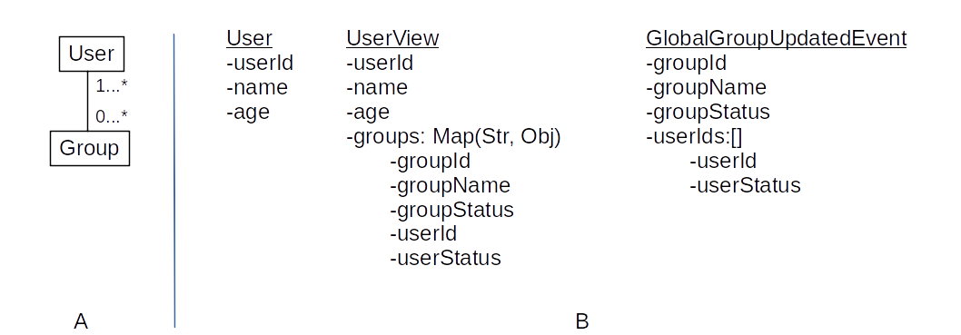
Fig. 4. Data model of Users service (A). User Aggregate, User View, Group Update Event (B)
To create a new user (Fig. 3), the REST controller receives a request (C-1). The controller sends a CreateUserCommand via a command bus to the AggregateService (C-2). The AggregateService calls the AggregateDAO to create and persist a new Aggregate (C-3); if positive, the AggregateService publishes a UserCreatedEvent with the new aggregate data.
The User event listener gets the event (C-4), broadcasts the event to the message broker, calls QueryService directly (C-5) to update the UserView (C-6). When the AMQP controller receives a GlobalGroupUpdatedEvent (Fig. 3, GU-1), the controller calls QueryService (GU-2) directly to update the UserView (GU-3).
Notice how an aggregate is updated in our case. Usually [MsPs, Ch. 5], to update an aggregate as a whole, a transaction is created. Within the transaction, an old aggregate is read, and the constraints of the old and the new aggregates are checked. If OK, the aggregate gets updated, and the transaction is committed.
If, however, it is permissible to send a whole aggregate to the front-end, then we can modify it there, check the constraints in the AggregateService, and finally, update the aggregate in the DB as a single document (with $set:{...user} command). No (explicitly created) transaction is needed, and all the aggregate’s constraints are satisfied.
Let’s summarize why the MERN stack with NestJS monorepo is very good for domain microservices:
- Typescript and monorepo make it easier to share the same DTO types, ts-rest contracts, code-first GraphQL annotated classes, and Zod-like schemes between a Typescript front (ReactJS) and back-end NestJS apps. To my knowledge, TSR doesn’t do this.
- MongoDB is great for CRUD nested objects, including maps; this is equally useful for dealing with both aggregates and views. For other scenarios, like audit, a graph DB can be better (Appendix C).
- CQRS efficiently deals with a lot of commands and queries. To my knowledge, TSR uses a simple three-layer architecture and a single read/write DB for CRUD operations.
- An extensive ecosystem with various communication technology modules (GraphQL, gRPC, RabbitMQ, Kafka,…) and architectural styles (CQRS) out of the box.
- Extensive testing and mocking utilities.
- NestJS CLI is useful to generate controller, module, CRUD resource, etc, boilerplate code and so possesses some TSR code generation capabilities.
Finally, let’s point out that domain services are the most often called from front-end apps. Some developers use LLMs to convert text and/or voice commands into API calls to domain services.
I believe, however, that this will not pay off: a thoughtfully made conventional UI with modern tech, like GraphQL, will work better than a hyped LLM functionality that regularly misinterprets requests. Let’s move to our DS/OR microservices.
Data Science/Operations Research Microservices
As was already mentioned, DS/OR microservices are less frequently called but have a complex input/output data format and unpredictably long computation time.
So, we don’t have to worry about running out of controller threads and can use a simpler three-layer architecture. The logic core methods are called directly, and a database is used to store intermediate results (later to train an ML-assisted mixed integer solver, for example).
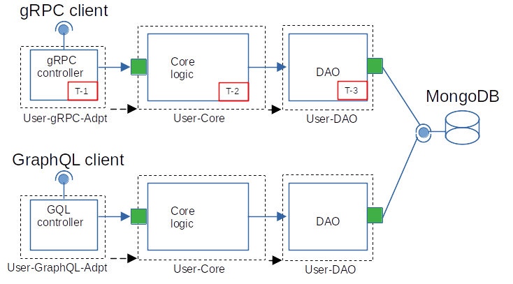
Fig. 5. DS/OR microservice architecture. The notation is the same as before.
Basically, DS/OR microservices have to process two kinds of scenarios: a request-response and a (near) real-time stream processing; the latter requires input-output stream RPCs.
Consider hexagonal Python microservices (Fig. 5), where every inbound adapter, as before, has an entry point if __name__ == '__main__'. Every inbound adapter imports a logic core that, in turn, imports a DAO module. Such apps may couple with each other via a common database.
A request first comes to an inbound adapter (T-1), then a logic method is called synchronously (T-2), intermediate results are persisted (T-3); finally, the logic method returns a result back to the inbound adapter.
I found gRPC to be the most useful communication technology for a DS/OR inbound adapter, for it can deal with complex input/output data formats via gRPC DSL and .proto files. Also, a gRPC input/output stream server is easy to program and set up. Other communication tech inbound adapters (GraphQL, REST, AMQP) are also implemented in the starter and may be useful in certain situations, when, for example, RabbitMQ infrastructure is already available.
These less common (in comparison to REST) communication technologies allow us to conveniently and efficiently integrate our DS/OR functionality into our common IS. Let’s take a closer look at the composer.
Composer
The composer follows the same hexagonal architecture outlined above. There is an inbound adapter to receive requests and core logic to process the requests in multiple steps (and to pull data from multiple sources); results are returned to the adapter and then to the user (Fig. 6). Since the requests are processed in multiple steps, it is nice to report progress status or intermediate results back to the user.

Fig. 6. Composer architecture. The notation is the same as before.
There are REST and GraphQL inbound adapters (separate Spring Boot apps, each with its own main method), and a core logic. As an inbound adapter receives a new request, the adapter calls a new task route. The route may “check the health” of the needed microservices and compose an execution plan (graph).
To build a plan, the new task route may call a specialized service to parse a request and build an execution graph on the fly. Then Camel conditional routing capabilities allow us to execute the task (in its simplest form it is demonstrated here). To my knowledge, TSR can’t build execution plans dynamically.
This plan is then executed step by step by other routes. In our case, the steps are REST, AMQP, gRPC, Result, and Stop. At every step, a piece of data is received from an outbound adapter and processed. Then, an intermediate result message is sent to the inbound adapter via a Reactor sink. These messages are disparate, so every route has a sink converter. The inbound adapter receives a message from the sink and streams the messages to the browser.
You might wonder if it would be easier to use a wiretap pattern in this case instead of a more complex Reactor sink. Indeed, such a composer would be more straightforward to build. However, in this case, the browser has to poll the composer periodically to obtain a task status.
The camel framework is especially useful for this kind of scenario. It has, among others, extensive data conversion, async processing, and routing tools. Useful documentation is also very handy.
Notice that since the composer calls a number of external RPCs, the calls need to be made asynchronously so that the system doesn’t consume CPU cycles while it waits for an RPC to reply. Builder, template method, and strategy design patterns make it easier to reuse code for different clients (REST, AMQP, gRPC in our case). Let’s see how exceptions are handled.
Exception Handling
Every real-life system faces problems, and so must have a way to handle them. Here, I implemented the following scheme (Fig. 7) whenever reasonable. Every module (controller, logic, DAO) has its own set of exceptions. Also, every module converts exceptions of its child modules into its own exceptions.

Fig. 7. Exception handling scheme of the starter
With monorepo architecture, it is easier to have a common exception set. Also, for microservices, we need to get and pass a correlation ID of every request to an exception’s message. Let’s see how to containerize the starter.
Dockerization
Let’s elaborate on how to dockerize the starter. Recall that every inbound adapter of every microservice is an entry point (with a main method), which imports a logic module as a library, which, in turn, imports a DAO module (also as a library).
Every such application is built as a separate image and deployed in its own container (Fig. 8). Notice that these apps (with the same logic and DAO) can also be deployed in a single container.
All the containers are run in a docker composer (DC) with a default network. As usual, for a DC, we set a container’s DC service name as a hostname to communicate with the service.

Fig. 8. How to dockerize the starter
Finally, let’s point out that every microservice (Spring Boot, NestJS, ReactJS-Vite, Python frameworks) requires its own procedure to build a docker image. ReactJS-Vite is especially quirky for a Vite builder sets the deploy parameters (like hosts and ports) into a compiled main.js file directly, so that the parameters are essentially fixed.
Conclusion
In this post, I presented a starter for a distributed multi-language analytics and information system with domain, data science, and composer services. Specifically, the starter demonstrates how to efficiently integrate data science and operations research functionality with a common information system.
Due to a versatile hexagonal architecture, the starter can be readily extended with other communication technologies and databases. Also, I pointed out how this system compares with LLM and TSR technologies.
Appendix A. Some Microservice Terminology
Here I follow [MsPs]:
Aggregate
A graph of objects that can be treated as a unit [MsPs, Ch. 5]. An aggregate contains a root entity and, possibly, one or more other entities and value objects; C/U/D functionalities deal with aggregates. Aggregates are only referenced by their roots. Inter-aggregate references must use primary keys instead of object references. Aggregates should be updated as a whole.
Composer Pattern (or API Composer) [MsPs, Ch. 7]
Implements a query operation by invoking the services that own the data and combining the results. Notice how a composer differs from a saga [MsPs, Ch. 6]: the later is a sequence of local transactions (that can roll back if unsuccessful).
CQRS Pattern [MsPs, Ch. 7]
Separate parts of the system and separate DBs to deal with Read (Query) and Create/Update/Delete requests (Command).
Domain
A noun (with, may be, child nouns) in user scenarios [MsPs, Ch. 2].
Domain Event
Notifies subscribers of changes to aggregates [MsPs, Ch. 5].
Entity
An object with a persistent identity.
Hexagonal Architecture
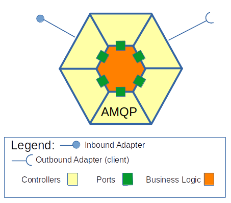
[MsPs, Ch. 2] this architectural style has one or more inbound adapters that handle requests from the outside by invoking the business logic (Fig. A). Similarly, the system has one or more outbound adapters that are invoked by the business logic and invoke external applications. Also, the business logic has one or more ports – a set of operations for the business logic to interact with adapters (in Java, ports may be Java interfaces).
The business logic doesn’t depend on the adapters, but the adapters do depend on the logic. This means that although an inbound adapter usually contains an entry point to a microservice (a main method in Spring boot, an app.listen() in NestJS), the adapter converts its data to “fit” into the business logic port.
Value Object
A collection of values.
View
A read-optimized DB or a virtual table (like in PostgreSQL).
Appendix B. Why OR and Predictive/Prescriptive Analytics Is Hard to Automate
According to [ZF], an OR pipeline is as follows:
- Problem identification and definition
- Parameter generation
- Model formulation
- Model optimization
- Interpretation and validation
The hardest step to automate here is 3.
As [ZF] points out, people currently try to use LLMs to convert text-based problem descriptions into mathematical models. The results on textbook problems are as follows: general purpose LLMs: 24-82% accuracy, OR tailored LLM (NL4OPT): up to 90% accuracy. So, for real-world problems, LLM formulations can serve only as a starting point for OR experts to create mathematical models.
An often overlooked fact is that linear and (even more so) mixed-integer programming problems are ill-posed (an output is highly sensitive to an input) [TA, Ch 9]. So, we can’t afford LLM formulation mistakes; every OR equation and constraint must be carefully examined. Special regularization algorithms can alleviate this problem, but only to an extent. See, for example, [Pan, Ch. 7], and [Vas, Ch. 4-5].
These LLM limitations for OR (and advanced analytical problems in general) are no accidents. According to [Bub], GPT-4 “can also make very basic [math] mistakes and occasionally produces incoherent output which may be interpreted as a lack of true understanding [of math].”
Appendix C. Document vs. Relational vs. Graph Databases
I found the following mental picture to keep in mind when to choose among document (DDB), relational (RDB), or graph data bases (GDB) (Fig. C). If your data model resembles “connected pyramids,” then consider a DDB. On Fig. C A, a document of Group collection refers to a document of User collection.
MongoDB, a DDB, is especially good in dealing with inheritance (via the discriminator mechanism). Also, MongoDB is good when a schema is not fully known in advance or very complex, like when you save intermediate results of complex computations. Finally, MongoDB now fully supports ACID transactions, and scales horizontally via sharding mechanism.

On the other hand, GDBs, like Neo4j, treat individual entities as graph nodes (graph edges can also carry information) (Fig. C C). These data bases are especially useful for “graph problems”, like to find indirectly connected entities, cycles, etc (see, for example, this post on audit functionality). Neo4j is also ACID — compliant and scales horizontally. A negative side of Neo4j is that it takes an order of magnitude more disk space.
Finally, RDBs, like PostgreSQL, are still the most widely used, constantly improving, with a huge community, and usually chosen by default unless there are special scenarios (like those described above) in your project. Of course, CAP theorem limits any hard-constraint database to scale horizontally.
Literature
- [Bub]: Sébastien Bubeck, Varun Chandrasekaran, Ronen Eldan, Johannes Gehrke, Eric Horvitz, Ece Kamar, Peter Lee, Yin Tat Lee, Yuanzhi Li, Scott Lundberg, Harsha Nori, Hamid Palangi, Marco Tulio Ribeiro, Yi Zhang, “Sparks of Artificial General Intelligence: Early experiments with GPT-4.”
- [MsPs]: Chris Richardson’s “Microservice patterns.”
- [Pan]: Ping-Qi Pan, “Linear Programming Computation.”
- [TA]: A.N. Tikhonov, V.Ya. Arsenin, “Solutions of ill-posed problems.”
- [Vas]: F.P. Vasilyev, A. Yu. Ivanitskiy, “In-depth analysis of linear programming.”
- [ZF]: Zhenan Fan, Bissan Ghaddar, Xinglu Wang, Linzi Xing, Yong Zhang, Zirui Zhou, “Artificial Intelligence for Operations Research: Revolutionizing the Operations Research Process.”
