Alternate encoder and dual decoder CNN-Transformer networks for medical image segmentation

Implementation details

The implementation of our proposed AD2Former was based on the PyTorch library and Python 3.8. The experiments were conducted on a single NVIDIA RTX 3090 GPU. In our experiments, we resized images to \(224\times 224\). In order to better initialize our model, we used a pre-trained ResNet34 model. After conducting a thorough comparon, we selected the following hyperparameters for each dataset:

• For Multi-organ Synapse datasets: We preprocessed the resolution of the original images to \(224\times 224\) size using rotation and flipping data augmentation techniques. The model was trained using the SGD optimizer with a batch size of 4 for 150 epochs, where the momentum was set to 0.9, the weight decay rate was 1e-4, and the learning rate was set to 0.01.

• For ISIC2018 datasets: Learning rate is set to 0.02, using the Adam optimizer to train for 150 epochs with a batch size of 4. The weight decay rate was 1e-4.

Evaluation metrics

We employ Dice score and Hausdorff Distance(HD) as evaluation metrics to measure the segmentation performance of the model on the Synapse dataset. For the skin lesion dataset, we used Dice score (DSC), specificity (SP), sensitivity (SE), and accuracy (ACC) to evaluate performance. The specific formulas are as follows:

Where FP and FN represent the number of foreground and background pixels that were predicted incorrectly. TP and TN represent the number of correctly classified foreground and background pixels. It should be emphasized that since the Synapse dataset consists of many classes, we must first get the DSC for each class before averaging the Dice scores for all classes to determine the final overall DSC. The formula for HD is:

Where h(X, Y) is defined as \(\underset{a\in A}{max}\{{\underset{b\in B}{min} \Vert x-y \Vert }\}\), and h(Y, X) is defined as \(\underset{b\in B}{max}\{{\underset{a\in A}{min} \Vert y-x \Vert }\}\), where X and Y represent the predicted and ground truth segmentation maps, x and y represent pixels in the predicted and ground truth maps, and \(||\cdot ||\) denotes the distance metric between x and y.

Ablation studies

To demonstrate the effectiveness of our proposed network, we conducted ablation studies that primarily focused on two aspects: the validity of the core module and the efficacy of the model parameters. Due to the limited space of the article, we conducted the main studies on the Synapse dataset and performed ablation studies to showcase the outstanding performance of our proposed network architecture.

Effectiveness of model parameters

To explore the optimal parameters, we studied the impact of the depth of the Transformer and the MLP size in each Transformer sub-module on the performance of the model and conducted two sets of ablation studies. For the three stages of using the ViT encoder, we used a layer list [\(l_1\), \(l_2\), \(l_3\)] to indicate the layer settings for the three Transformer modules in the encoder. For the MLP size, we compared our model with the original dimensionality expansion factor and used M to represent the dimensionality expansion factor of the first fully connected layer in the MLP block of the Transformer. The specific results of different configurations are shown in Table 1 and Table 2. The results show that using 3/3/3 configuration for the depth of the Transformer layers in the three stages achieves the best performance. The experimental results indicate that although the depth of the Transformer layers was increased in the second and third stages, it did not lead to a significant improvement in segmentation accuracy. It can also be seen that an MLP block with an expansion factor of \(M=2\) performs better than the DSC values of other configurations, bringing 1.36% performance improvement.

Validity of core modules

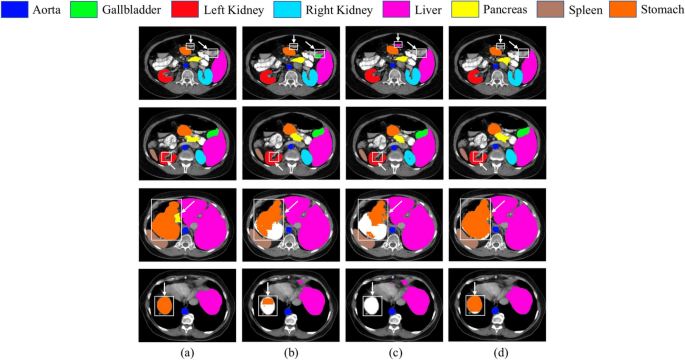
In this section, we first validate the effectiveness of CFB. The objective of the ablation study was to test how changing the number of skipping connections in CFB would affect its performance. We compared the results of skip-0 (no CFB), skip-1 (ours), and skip-2. The experimental results are presented in Table 3. Our findings demonstrate that adding skip-1 to CFB increased the DSC by 1.26 \(\%\), resulting in the best performance. However, the performance decreased when skip-2 was added. This is mainly because more skip connections introduce noise, which degrades the impact of each connection’s information transmission. To more clearly illustrate the impact of different numbers of skip connections on segmentation performance, we conducted three approaches with different numbers of skip connections on the Synapse dataset and presented the comparison results in Fig. 5.

For example, in the first row of segmentation results, skip-0 and skip-2 frequently misclassify background information as foreground. But our skip-1 approach demonstrates accurate pixel classification in the vicinity of the target area. In the second row, skip-1 segments the edge data in the segmentation region more accurately. In the third and fourth rows, when compared with the Ground Truth, we can clearly see that skip-1(ours) performs better than the other two approaches in the segmentation of the stomach. skip-0 fails to detect some regions in the third row, while skip-2 only captures a small portion of the stomach, However, our skip-1 effectively identifies the majority of the area.

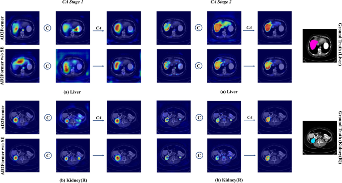
Furthermore, we conducted ablation studies to examine the effectiveness of the channel attention module, as shown in Table 4. The experiments demonstrated that AD2Former outperformed AD2Former w/o CAM, achieving an average DSC improvement of 0.54\(\%\). This result suggests that without the channel attention module, directly fusing the CNNs and transformer feature maps at the same scale outputted by DUD through a \(3\times 3\) convolution and inputting them to CFB may cause feature redundancy, which can affect the segmentation performance. By adding the channel attention module, the network learned the correlation between feature channels, making the extraction and utilization of local and global information more effective. To compare the feature learning performance of the model with and without the channel attention module graphically, we show the key feature maps of the two approaches as shown in Fig. 4. We created maps of the liver and right kidney’s before- and after-channel attention features. We found that the network could concentrate more on the target organ area when the CAM module was applied in the initial stage of segmentation. In the second stage, compared to the situation without the channel attention module, our model was better able to pay attention to semantic information. For the right kidney segmentation, in stage1, although the features generated by the ViT sub-decoders misclassify the left kidney as the right kidney, the feature selection through channel attention allows for a greater focus on the region corresponding to the right kidney.

Results of multi-organ segmentation

To validate the superiority of our proposed method in multi-organ image segmentation tasks, we compared it with the current state-of-the-art methods based on CNN and Transformer. To ensure the relative consistency of the experimental results, we conducted comparative experiments under the same experimental settings. The results are shown in Table 5. The best results are highlighted in black bold. It should be noted that AD2former is a framework for 2D images, so only the 2D network is compared in the comparison process, not the 3D network.

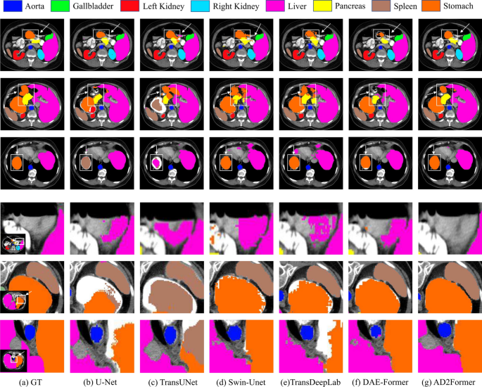
As presented in Table 5, our AD2Former outperformed other network architectures with DSC of 83.18\(\%\) and HD of 20.89\(\%\). Moreover, our method achieved the best performance for liver, pancreas, spleen, and stomach segmentation. Specifically, in the segmentation of the pancreas and stomach, our method outperformed the second-best methods MISSFormer ¹⁸ and HiFormer ²⁵ by 4.04\(\%\) and 3.15\(\%\), respectively. In order to further illustrate the merits of our proposed approach, a paired student’s t-test was carried out in comparison with the second set of results. The obtained p-value (p<0.05) clearly demonstrates a statistically significant distinction between our method and those of the comparison. We also conducted a visual comparison of different methods on the Synapse dataset. We randomly selected six slices and divided them into two groups. One group was used to compare the overall segmentation effect, while the other group was used to observe the segmentation effect at the edges, as shown in Figure 7. It can be seen from the first group of slices (the first three rows), our method achieved better organ segmentation performance when compared with the other five networks. Compared to CNN-based methods, transformer-based methods pay more attention to the global context information but have some limitations in handling local details, especially in accurately judging the details on the edges of the segmentation region. As shown in the second row, other model misclassified the peripheral background information of the liver and stomach as foreground information. Although DAE-Former combines self-attention and convolution, it still has certain issues in handling boundary information, such as misclassifying parts of the boundaries of the pancreas and stomach in the image. In contrast, our proposed AD2Former model, through the real-time interaction of self-attention and convolution mechanisms and dual decoding process, can more accurately classify the information of the pancreas and stomach. In the second group of slices, taking the first row as an example, other models would misclassify irrelevant regions as the liver, while our proposed model performs excellently and is completely unaffected by such interferences. In the second row, when faced with highly blurred edges, other models struggle to achieve precise segmentation, with jagged and indistinct segmentation lines. In contrast, the AD2Former model can, by virtue of its outstanding performance, delineate organ edges relatively clearly, with distinct segmentation boundaries.

However, there are also some failed cases worthy of discussion during the segmentation process. As shown in the Figure 6, when the samples are severely imbalanced, the model may also encounter inaccurate segmentation situations.

Results of skin lesion segmentation

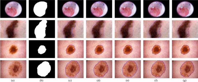
We also evaluated the performance of AD2Former on the ISIC2018 skin lesion dataset and compared it with existing state-of-the-art (SOTA) approaches to demonstrate the generalizability. All of the competitors were tested under the same computing environment. Table 6 shows the accuracy (ACC), sensitivity (SE), specificity (SP), Inference Speed(Images/S), Memory Utilization and Dice score (DSC) of each method. Our method clearly outperformed other image segmentation networks in all indices, achieving the highest DSC and SE scores of 91.28\(\%\) and 92.00\(\%\), SP and ACC also have the highest scores, with 98.82\(\%\) and 96.49\(\%\), respectively. The Inference Speed refers to the number of pictures that can be inferred per second. On average, the AD2Former can infer 36 pictures per second, and the memory usage rate during training reaches 99%. Furthermore, the p-value(p<0.05) based on student’s T-test indicates that our method is significantly different from these comparative methods. The comparison with attention-based methods further shows that our method has better robustness and generalization ability. Furthermore, we conducted a visual comparison of the segmentation results of different models. In our experiments, we selected U-Net, TransUNet, FAT-Net, and Swin-Unet as representative methods for visual comparison, as shown in Figure 8. The best results are highlighted in black bold.

Based on our observations, our method generally outperforms other competitors and achieves the best segmentation results. U-Net struggles to distinguish foreground information from background information without global context information, leading to inaccurate predictions when handling skin lesion edges. Although FAT-Net combines global and local information to reduce the impact of weak global context information extraction ability, it can be too sensitive and result in a larger prediction range, thereby reducing its accuracy. Swin-Unet introduces a window mechanism to reduce computational complexity, but it still has insufficient global information interaction, particularly when dealing with samples with complex boundaries, causing mis-segmentation. However, our model adopts an alternating learning strategy, which can overcome the deficiency of insufficient local and global interaction. The operation of dual encoders can optimize detail information, enabling our model to better cope with challenging scenarios like low contrast, blurred boundaries, and so on. Therefore, as shown in the figure above, our model can achieve better segmentation results than other competitors in such cases.