Deep representation learning for clustering longitudinal survival data from electronic health records

EHR dataset from UK Biobank

This study was conducted using the UK Biobank resource, which has ethical approval and its own ethics committee (https://www.ukbiobank.ac.uk/ethics/). This research has been conducted using UK Biobank resources under Application Number 57952. For our analyses, we used both the primary and hospital inpatient care diagnosis records made available via the UK Biobank study⁶⁴. We started from 451,265 patients with available hospital inpatient care data. For each patient, a diagnosis sequence was constructed by interleaving the hospital inpatient care data with any available primary care data based on their timestamps. We then mapped all resulting diagnosis codes from Read v2/3 and ICD-9 to ICD-10⁶⁴. For those codes mapping to multiple ICD-10 codes, we included all possible mappings. Keeping only patients with at least five diagnoses, at most 200 diagnoses, and at least one month of diagnosis history, the resulting dataset consisted of 352,891 patients.

The data processing pipeline is visualized in Supplementary Fig. 16, and the resulting dataset is summarized in Table 1, Supplementary Table 1, and Supplementary Fig. 1.

VaDeSC-EHR architecture

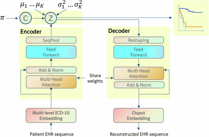
For implementing VaDeSC-EHR, we integrated VaDeSC into a transformer-based encoder/decoder architecture for learning patient representations (Fig. 1). Here, we describe the architecture and generative process in more detail.

The generative process

Adopting the approach of VaDeSC²¹, first, a cluster assignment \(c\in \left\{\left.2,\ldots,K\right\}\right.\) is sampled from a categorical distribution: \(p\left(c\right)={Cat}\left(\pi \right)\). Then a latent embedding \(z\) is sampled from a Gaussian distribution: \(p\left(z|c\right){{=}}{{{\mathcal{N}}}}\left({\mu }_{c},{\sigma }_{c}^{2}\right)\). The diagnosis sequence \(x\) is generated from \(p\left(x|z\right)\), which for VaDeSC-EHR is modeled by a transformer-based decoder as described below. Finally, the survival time \(t\) is generated by \(p\left(t|z,c\right)\).

Transformer-based encoder and decoder

Embedding

First, for each ICD-10 code, its subcategory (e.g. K50.1), category (e.g. K50), and block (e.g. K50-K52) were extracted using the algorithm shown in Supplementary Note 1.

Then, the ICD-10 code (subcategory, category, and block), age, and type (primary or hospital) were individually embedded, while adding a sinusoidal position embedding to each of the individual embeddings. The position embedding was based on the visit number of the diagnosis within the diagnosis sequence⁶. Hence, diagnoses originating from the same doctor’s visit received the same position embedding. Finally, the individual embeddings were summed to arrive at the final embedding for each diagnosis (Fig. 2):

Encoder

The embeddings were fed into a classical transformer encoder^6,7 augmented with a SeqPool layer⁶⁵ to consolidate the entire sequence of a patient into a single comprehensive representation for that individual. More specifically, given:

where \({X}_{L}\) is the output of an \(L\) layer transformer encoder \(f\), and \(b\) is the batch size, \(n\) is the sequence length, \(d\) is the total embedding dimension. \({X}_{L}\) was fed into a linear layer \(g({X}_{L})\in {{\mathbb{R}}}^{d\times 1}\), and a softmax activation was applied to the output:

This generated an importance weighting for each input token, which was used as follows⁶⁵:

By flattening, the output \(z\in {{\mathbb{R}}}^{b\times d}\) was produced, a summarized embedding for the full patient sequence.

Decoder

First, the latent representation was transformed using fully connected layers:

Here, \(i\) is the number of layers, \(b\) the batch size, \(L\) the sequence length, \(J\) the number of latent variables, \(H\) the dimensionality of embedding, and \(Z\) the latent representation (Fig. 1).

\(X\) was then reshaped to \({X}_{{re}}\) (\({{\mathbb{R}}}^{b\times {LH}}\to {{\mathbb{R}}}^{b\times L\times H}\)) and fed into the transformer decoder^6,7 to generate the reconstructed ICD embedding \({\hat{E}}_{{ICD}}={{{\rm{Decoder}}}}({X}_{{re}})\). The reconstructed input embedding for each diagnosis for a given patient was then computed as:

Here, \({E}_{{age}}\), \({E}_{{type}}\) and \({E}_{{position}}\) were copied over from the input to the transformer encoder.

Finally, the original EHR input sequence (up to the level of the ICD-10 subcategory) was reconstructed from \({E}_{{decoder}}\) using a softmax function.

Evidence lower bound (ELBO)

The loss on the architecture as described above was computed using the ELBO as previously defined for VaDeSC by Manduchi et al.²¹. We briefly present the formula and outline its interpretation, but for more details, we refer the reader to Manduchi et al.²¹.

The ELBO of the classic VAE²² looks as follows:

Here, \(x\) is the input patient diagnosis sequence, \(z\) is the latent space for the patient. The first term \(p\left(x|z\right)\) can be interpreted as the reconstruction loss of the autoencoder. In the second term, \(q\left(z|x\right)\) is the variational approximation to the intractable posterior \(p\left(z|x\right)\) and can be seen as regularizing z to lie on a multivariate Gaussian manifold²².

Adding a cluster indicator as in VaDE²³, the ELBO looks as follows:

The first term is the same as above. Analogous to the above, in the second term, \(q\left(z,c|x\right)\) is the variational approximation to the intractable posterior \(p\left(z,c|x\right)\) and can be seen as regularizing \(z\) to lie on a multivariate Gaussian mixture manifold.

Finally, additionally, including a survival time variable t in the model as in VaDeSC²¹, the ELBO looks as follows:

The reconstruction loss \(p\left(x|z\right)\) is calculated as sequence length*mean cross-entropy.

The survival time \(p\left(t|z,c\right)\) is modeled by a Weibull distribution and adjusts for right-censoring:

Here, the variable \(\delta\) represents the censoring indicator, which is assigned 0 when the survival time of the patient is censored, and 1 in all other cases. For each patient, given by the latent space \(z\) and cluster assignment \(c\), the uncensored survival time is assumed to follow a Weibull distribution: \(f\left(t\right)={Weilbull}\left({\lambda }_{c}^{z},k\right)=\frac{k}{{\lambda }_{c}^{z}}{(\frac{t}{{\lambda }_{c}^{z}})}^{k-1}\exp (-{(\frac{t}{{\lambda }_{c}^{z}})}^{k})\), where \({\lambda }_{c}^{z}={softplus}({z}^{T}{\beta }_{c})\), \({\beta }_{c}\in \left\{\left.{\beta }_{1},{\beta }_{2},\ldots,{\beta }_{K}\right\}\right.\). The censored survival time is then described by the survival function \(S\left(t|z,c\right)=\exp (-{(\frac{t}{{\lambda }_{c}^{z}})}^{k})\).

For more details and the complete derivation of the VaDeSC ELBO, we refer the reader to Manduchi et al.²¹.

Pre-training and fine-tuning strategy

For the real-world data applications (diabetes and CD), we first pre-trained the transformer encoder on the entire UK Biobank EHR dataset (Table 1, column 3). Following the original BERT study, we used a masked diagnosis learning strategy for pre-training. Specifically, for each patient’s diagnosis sequence, we set an 80% probability of replacing a code by [MASK], a 10% probability of replacing a code by a random other code, and the remaining 10% probability of keeping the code unchanged. The ICD-10 embeddings were randomly initialized, and the encoder was trained using an Adam optimizer with default beta1 and beta2.

For selecting our final transformer architecture, we followed the Bayesian hyperparameter optimization strategy as described in the BEHRT study⁴. The best-performing architecture consisted of 6 layers, 16 attention heads, a 768-dimensional latent space, and 1280-dimensional intermediate layers (more details in Supplementary Table 2).

After transformer encoder pre-training, we fine-tuned VaDeSC-EHR end-to-end on the T1D/T2D dataset (Table 1, column 4) and the CD dataset (Table 1, column 5). Details around fine-tuning are described in the following section.

VaDeSC-EHR in various applications

Synthetic benchmark

Data generation

We used a transformer decoder with random weights to simulate diagnosis sequences (Supplementary Fig. 2). More specifically, let \(K\) be the number of clusters, \(N\) the number of data points, \(L\) the capped sequence length, \(H\) the dimensionality of embedding, \(D\) the size of vocabulary, \(J\) the number of latent variables, \(k\) the shape parameter of the Weibull distribution and \({p}_{{cens}}\) the probability of censoring. Then, the data-generating process can be summarized as follows:

1. 1.

   Let \({\pi }_{c}=\frac{1}{K}\), for \(1\le c\le K\)

2. 2.

   Sample \({c}_{i} \sim {Cat}\left(\pi \right),\) for \(1\le i\le N\)

3. 3.

   Sample \({\mu }_{c,j} \sim {unif}\left(-{10,10}\right),\) for \(1\le c\le K\) and \(1\le j\le J\)

4. 4.

   Sample \({z}_{i}{\sim}{{{\mathcal{N}}}}({\mu }_{{c}_{i}},{\varSigma }_{{c}_{i}})\), for \(1\le i\le N\)

5. 5.

   Sample \({{seq}}_{i} \sim {unif}\left(0,L\right),\) for \(1\le i\le N\)

6. 6.

   Let \({g}_{{res}}\left(z\right)={reshape}\left({ReLU}\left({wz}+b\right),L\times H\right)\), where \(w\in {{\mathbb{R}}}^{{LH}\times J}\) and \(b\in {{\mathbb{R}}}^{{LH}}\) random matrices and vectors.

7. 7.

   Let \({x}_{i}={g}_{{res}}({z}_{i}),\) for \(1\le i\le N\)

8. 8.

   Let\(\,{g}_{{att}}\left(x\right)={softmax} (\frac{\left({w}_{Q}x+{b}_{Q}\right){\left({w}_{K}x+{b}_{K}\right)}^{T}}{\sqrt{H}}+{mask} )\left({w}_{V}x+{b}_{V}\right),\) where \({w}_{Q}\), \({w}_{K},{w}_{V}\) and \({b}_{Q},{b}_{K},{b}_{V}\) are random matrices and vectors. Mask is based on \({{seq}}_{i}\)

9. 9.

   Let \({x}_{i}={g}_{{att}}({g}_{{att}}({g}_{{att}}({x}_{i}))),\) for \(1\le i\le N\)

10. 10.

    Let\({g}_{{dec}}(x)={softmax}({ReLU}({wx}+{b})),\) where \(w\in {{\mathbb{R}}}^{D\times H}\) and \(b\in {{\mathbb{R}}}^{D}\) random matrices and vectors.

11. 11.

    Let \({x}_{i}={argmax}({g}_{{dec}}({x}_{i}))[1:{{seq}}_{i}],\) for \(1\le i\le N\)

12. 12.

    Sample \({\beta }_{c,j} \sim {unif}\left(-{{\mathrm{2.5,2.5}}}\right),\) for \(1\le c\le K\) and \(1\le j\le J\)

13. 13.

    Sample \({u}_{i} \sim {Weibull}({softplus}({z}_{i}^{T}{\beta }_{{c}_{i}}),k)\), for \(1\le i\le N\)

14. 14.

    Sample \({\delta }_{i} \sim {Bernoulli}(1-{p}_{{cens}}),\) for \(1\le i\le N\)

15. 15.

    Let \({t}_{i}={u}_{i},\) if \({\delta }_{i}=1,\) and sample \({t}_{i} \sim {unif}\left(0,{u}_{i}\right)\) otherwise, for \(1\le i\le N\)

In our experiments, we fixed \(K=3,N=30000,J=5,D=1998\) (ICD-10 category-level vocabulary)\(,k=1,{p}_{{cens}}=0.3,\) \(L=100.\) For the attention operation, we used 3 attention layers with 10 heads in each layer.

Model training and hyperparameter optimization

Hyperparameter optimization was done by a grid search on learning rate ({0.1, 0.05, 0.01, 0.005, 0.001}) and weight decay ({0.1, 0.05, 0.01, 0.005, 0.001}), using an Adam optimizer with default beta1 and beta2. For performance estimation, we split the generated data into three parts, one-third for training, one-third for validating, and one-third for testing the model. We repeated the above 5 times (i.e. for 5 randomly generated datasets) to arrive at a robust average performance estimate.

Real-world diabetes benchmark

Data extraction

To extract the data, we selected patients by the occurrence of ICD-10 codes E10 (T1D) or E11.3 (T2D) in their diagnosis trajectories and labeled patients by the presence of H36 (“Retinal disorders in diseases classified elsewhere”). Because of sample size limitations, no requirement was placed on the minimum number of occurrences of each of E10 and E11.3. In order to avoid ambiguity in the performance estimation, patients with both E10 and E11 in their disease history were excluded, which resulted in the dataset as summarized in Table 4, column 2. In the training data, all occurrences of E10, E11, and H36 (and their children) were deleted to avoid data leakage. The selected patients substantially fitted the validated phenotype definition⁶⁶.

Model training and hyperparameter optimization

We fine-tuned VaDeSC-EHR end-to-end on the dataset described above, taking our pre-trained encoder as a starting point. Note that in the fine-tuning stage, the decoder could benefit from the pre-trained encoder, because weights were shared between the two. We used nested cross-validation (NCV)³⁰ with a 4-fold inner loop for hyperparameter optimization and a 5-fold outer loop for performance estimation. Hyperparameters were optimized using Bayesian optimization on the following hyperparameter grid:

• learning rate of the Adam optimizer: {1e-5, 5e-5, 1e-4, 5e-4,1e-3},

• weight decay parameters of the Adam optimizer: {1e-6, 1e-5, 1e-4, 1e-3, 1e-2, 0.1},

• dimension of latent variables: {5,10,15,20},

• shape parameter of the Weibull distribution: {1, 2, 3, 4, 5},

• dropout rate: {0.1, 0.2, 0.3, 0.4, 0.5},

• number of reshape layers: {1, 2, 3, 4, 5}.

Application: progression of Crohn’s disease toward intestinal obstruction

Data extraction

To extract the Crohn’s disease (CD) patient population, we selected patients by requiring at least one occurrence of the ICD-10 code K50 (Crohn’s disease) while excluding patients with a K51 diagnosis (ulcerative colitis) and then labeled patients according to the presence of K56 (“Paralytic ileus and intestinal obstruction without hernia”). This resulted in the dataset summarized in Table 4, column 5. In the training data, all occurrences of K50 and K56 (and their children) were deleted to avoid data leakage. The selected patients substantially fitted the validated phenotype definition⁶⁶.

Model training and hyperparameter optimization

We fine-tuned VaDeSC-EHR end-to-end on the dataset described above, taking our pre-trained encoder as a starting point. Note that in the fine-tuning stage, the decoder could benefit from the pre-trained encoder, because weights were shared between the two. We used the pre-trained encoder as the initial weight. And applied 5-fold cross-validation for hyperparameter optimization. Hyperparameters were optimized using Bayesian optimization, with a hyperparameter search space defined as for the diabetes model, except that we now also needed to optimize the number of clusters \(\left\{\left.2,\ldots,K\right\}\right.\) jointly with the other hyperparameters, because a ground-truth clustering was not available (\(K=4\), in this use case). The best combination of hyperparameters (including the number of clusters) was determined by encouraging a low Bayesian information criterion (BIC) and a high concordance index (CI) through maximizing: \(\sqrt{{{CI}}^{2}+{\left(1-{{BIC}}_{{norm}}\right)}^{2}}\), where the BIC was normalized to the interval [0, 1] (Supplementary Fig. 17, Supplementary Table 3).

Methods comparison and metrics

We compared VaDeSC-EHR to a range of baseline methods: variational deep survival clustering with a multilayer perceptron (VaDeSC-MLP), semi-supervised clustering (SSC)¹⁷, survival cluster analysis (SCA)¹⁸, deep survival machines (DSM)¹⁹, and recurrent neural network-based DSM (RDSM)²⁰, as well as k-means and regularized Cox PH as naïve baselines. In addition, to assess the influence of the survival loss on the eventual clustering, we included VaDeSC-EHR_nosurv, in which the survival loss of VaDeSC-EHR was turned off. Finally, to assess the influence of absolute age on distinguishing between ground-truth clusters, we included VaDeSC-EHR_relage (with age at first diagnosis subtracted from all elements in the age sequence). We used ICD-10-based TF-IDF features as the input for all methods but RDSM and VaDeSC-EHR, which allow for directly modeling sequences of events.

We evaluated the clustering performance of models, when possible, in terms of balanced accuracy (ACC), normalized mutual information (NMI), adjusted Rand index (ARI), and area under the receiver-operating characteristic (AUC). Clustering accuracy was computed by using the Hungarian algorithm for mapping between cluster predictions and ground-truth labels⁶⁷. The statistical significance of performance difference was determined using the Mann–Whitney U test.

For the time-to-event predictions, we used the concordance index (CI) to evaluate the ability of the methods to rank patients by their event risk. Given observed survival times \({t}_{i}\), predicted risk scores \({\delta }_{i}\), and censoring indicators \({\delta }_{i}\), the concordance index was defined as

Visualization and enrichment analysis of clusters

The clusters were visualized using UMAP (uniform manifold approximation and projection)⁶⁸ with the Jensen–Shannon divergence⁶⁹ as a distance measure: \({JSD}(P(c|{x}_{i}),P(c|{x}_{j}))\), where \(P\left(c|x\right)\) is the distribution across clusters c given a patient x. Cluster cohesion was measured using the silhouette coefficient⁷⁰.

We assessed the association of the clustering with sex, age, education level, location of UKB recruitment, 4 genetic principal components, fraction of hospital care data, and overall diagnosis sequence length using a Chi-squared test or a one-way ANOVA. We calculated the differential enrichment of diagnoses between clusters in two ways: (1) for individual diagnoses, and (2) for sequences of diagnoses. For the individual diagnoses, we used the ICD-10 codes as provided by the UK Biobank. For the diagnosis sequences, we first mapped the ICD-10 codes to Phecode⁷¹ and CALIBER codes⁷², which provided a higher level of abstraction in defining diseases. For each patient, we then identified all, potentially gapped, subsequences of three diagnoses from the EHR data, with the following constraints: (1) for duplicate diagnoses in the diagnosis sequence, we only considered the first one, (2) the subsequence contained a diagnosis of the disease under study (CD) but did not contain the selected risk event (intestinal obstruction).

We assessed the statistical significance of the differential enrichment using logistic regression models predicting patient clusters from subsequence occurrence while adjusting for the effects of age, sex, PC1, recruitment location, and fraction of hospital care data by including these variables as covariates into the model. We corrected the resulting p-values for multiple testing using the Benjamini–Hochberg procedure and set a threshold at 0.05 for statistical significance.

Analysis of smoking behavior

We analyzed the association of smoking behavior with progression toward intestinal obstruction using multivariate Cox regression models, individually testing the hazard ratio of several variables related to smoking behavior:

1. 1.

   data field 20160 (“Ever smoked”),

2. 2.

   diagnosis ICD-10 code F17.2 (“Mental and behavioral disorders due to use of tobacco dependence syndrome”), which is commonly interpreted as nicotine dependence⁷³,

3. 3.

   data field 20161 (“Pack years of smoking”),

4. 4.

   data field 20162 (“Pack years adult smoking as a proportion of life span exposed to smoking”),

5. 5.

   Current smoking status, which we defined as the union of patients identified as current smokers from data fields 1239 (“Current tobacco smoking”) and 20116 (“Smoking status”)

6. 6.

   Previous smoking status, which we defined as patients who had ever smoked but are not currently smoking. Additionally, to make sure the patients were not smoking at the time of their first CD diagnosis, we excluded patients whose assessment date was after the date of their first CD diagnosis.

The UK Biobank data fields we used contained data collected between 2006 and 2010.

We adjusted the above models for the effects of age, sex, PC1, recruitment location, fraction of hospital care data, and time difference between the CD onset and the nearest smoking diagnosis (F17.2) or assessment date, by including these variables as covariates in the model.

Genetic analysis of patient clusters

We computed pathway-based polygenic risk scores (‘pathway PRSs’ henceforth) using PRSet⁷⁴ to assess genetic differences between the patient clusters, restricting ourselves to UK Biobank participants of European ancestry⁷⁴. Quality control steps were performed before calculating pathway PRSs, including filtering of SNPs with genotype missingness > 0.05, minor allele frequency (MAF) < 0.01, and with Hardy–Weinberg Equilibrium (HWE) p-value < 5 × 10⁻⁸. We focused on 164 biological pathways related to Crohn’s disease as retrieved from the Gene Ontology – Biological Process (GO-BP) database, selected based on a literature and keyword search (“IMMUNE”) (Table S1)^75,76. We calculated pathway PRSs for each (patient, pathway) pair using variants located in exon regions. For each pathway PRS, we then fitted a logistic regression model predicting cluster from pathway PRS, while adjusting for age, sex, PC1, recruitment location, and the fraction of hospital care data. The p-value of the resulting coefficient was calculated using a log-likelihood ratio test⁷⁷ and corrected for multiple testing using the Benjamini–Hochberg procedure. For determining statistical significance, we used a threshold of 0.05.

After the pathway-level analysis, we extracted the individual genetic variants contributing to the pathway PRS. We applied Chi-squared tests to identify the significant SNPs⁷⁸ and corrected the resulting p-values for multiple testing using the Benjamini–Hochberg procedure. Finally, we fitted logistic regression models predicting cluster from mutation status, while adjusting for confounding by including age, sex, PC1, recruitment location, and the fraction of hospital care data as covariates in the models. We defined mutation status by dominant coding, thereby comparing no copy of the risk allele to at least one copy.

Reporting summary

Further information on research design is available in the Nature Portfolio Reporting Summary linked to this article.