SVLearn: a dual-reference machine learning approach enables accurate cross-species genotyping of structural variants

Sequencing data collection

Sequencing data used throughout this study were sourced from publicly available databases. A total of 45 individuals were collected, of which 15 human individuals were obtained from the Human Pangenome Reference Consortium³⁵, 15 sheep individuals were derived from a sheep pangenome study²², and 15 cattle individuals were obtained from five different studies (Charolais³⁶, Holstein³⁷, NxB and OxO³⁸, Yunling³⁹, the remaining ten individuals²¹). Each individual includes PacBio HiFi long reads and 2×150 bp paired-end short reads (Supplementary Table 1).

Construction of ground truth sets for SV genotypes

Minimap2⁴⁰ (version 2.26) was used to align the PacBio HiFi long reads of each human individual to the reference genome GRCh38 (https://ftp.ncbi.nlm.nih.gov/1000genomes/ftp/technical/reference/GRCh38_reference_genome/GRCh38_full_analysis_set_plus_decoy_hla.fa). Subsequently, we used Sniffles2⁴¹ (version 2.2) in multi-sample mode with parameter –minsupport 4 to derive SVs and their genotypes across 15 human individuals. We retained only the insertions and deletions within the range between 50 bp and 1 Mb on the chromosomes (autosomes and XY). To curate high-quality data, we removed any two SVs that were separated by less than 300 bp. This arises from the fact that closely arranged SVs are often characterized intricately and thus difficult to detect by computational methods^17,35,42. SVs with missing genotypes in any individual were also removed, resulting in the Human SV Set containing genotypes for all 15 individuals. We applied the same procedure to obtain SVs and their genotypes for 15 cattle and 15 sheep individuals using PacBio HiFi long reads, generating the Cattle SV Set and Sheep SV Set, respectively. The reference genome ARS-UCD1.2 (GCF_002263795.1) was used for mapping cattle individuals, while ARS-UI_Ramb_v2.0 (GCF_016772045.1) was used for mapping sheep individuals.

For genotyping performance comparison, we additionally derived SVs and their genotypes based on haplotype-resolved genomes of 15 human individuals. We downloaded haplotype-resolved genomes of the 15 human individuals from the Human Pangenome Reference Consortium (HPRC)³⁵. First, we excluded potentially contaminated contigs based on a previously published list (https://github.com/human-pangenomics/HPP_Year1_Assemblies/blob/main/genbank_changes/y1_genbank_remaining_potential_contamination.txt). Next, we called SVs and their genotypes using PAV¹⁷ (version 2.3.4) with default parameters, which were then merged using Jasmine⁴³ (version 1.1.5). The parameters for Jasmine are provided in the Supplementary Methods. Quality control was subsequently performed using the same criteria applied to the Human SV Set. After removing those SVs overlapped with genomic gap regions, we were left with a total of 39,746 SVs and the genotypes (referred to as the Human Assembly-based SV Set).

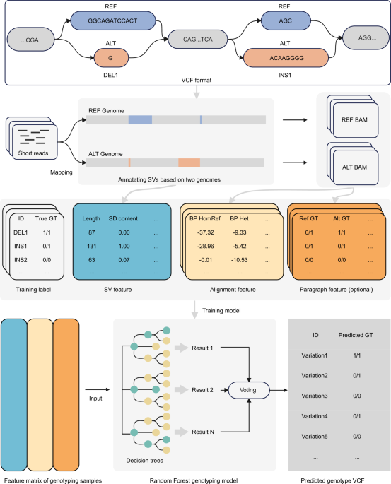
Generation of ALT genome

An ALT sequence from the ATL genome was constructed by applying alterations induced by SVs to its corresponding REF sequence from the REF genome. A genomic segment can be overwhelmed by multiple SV events detected from different individuals, such as those 2 small-sized deletions overlapped with 1 large-sized deletion (Supplementary Fig. 1). These overlapping SVs can create multi-allelic bubbles^35,44, thereby undermining the fidelity of SVs as biallelic. To avoid this, we devised two strategies, threshold-based and pseudo-contig-based sequence assemblies, to generate ALT sequences.

Using the threshold-based strategy, SVs occurring in a REF sequence are classified as either overlapping or non-overlapping. An SV is considered as non-overlapping if there exists a distance of at least 300 bp between the SV and each of its adjacent SVs. Finally, only non-overlapped SVs are utilized to construct each ALT sequence. However, this strategy often leads to a significant decrease in the number of SVs retained for assembling the ALT genome. For instance, in dataset “variants_GRCh38_sv_insdel_alt_HGSVC2024v1.0”, we were left with 51,110 SVs, less than one third of the raw SVs.

To maximize the retention of SVs, we employed the pseudo-contig-based strategy (Supplementary Fig. 1b), which builds a primary ALT sequence and several pseudo-contigs based on a single REF sequence containing overlapped SVs. The primary sequence was built by replacing the reference sequence at the leftmost overlapped SV (such as DEL2) with its ALT allele. Then, for each of the other overlapped SVs, a pseudo-contig (such as DEL3 and DEL4) for a deletion was built by concatenating 150 bp of flanking sequences on both the upstream and downstream sides of the deletion together, while a pseudo-contig for an insertion (such as INS3) was built by truncating the insertion and incorporating 150 bp of flanking sequences on each side. This approach effectively prevents the overwriting of previously replaced segments on the main chromosome and minimizes disruptions to read alignment.

Finally, genomic positions of the ALT sequences were recorded. Using the ALT sequence and positional information, BED and VCF files of SVs were then produced.

Short reads mapping

Short reads were mapped to the REF and ALT genomes using BWA-MEM2⁴⁵ (version 2.2.1) and the mapped reads in the BAM files were sorted using SAMtools⁴⁶ (version 1.17). PCR duplicates were removed using Sambamba⁴⁷ (version 1.0.1) by setting parameter markdup to -r, yielding BAM files for the two genomes, respectively. The CRAM files aligned to GRCh38 were downloaded for 14 of the 15 human individuals, except for HG002. Subsequently, SAMtools was used to convert the CRAM to BAM. Bazam⁴⁸ (version 1.0.1) was employed to extract short reads from the BAM files and remap them to the ALT genome. Mosdepth⁴⁹ (version 0.3.6) was utilized to calculate the coverage of both short and long reads with parameters –fast-mode –no-per-base –by 300. We analyzed short reads mapped to SV sites in reference (REF) and alternative (ALT) BAM files for 15 human individuals under 30× coverage. During the counting process, we excluded secondary alignments, PCR duplicates, and reads with a mapping quality of zero, as these reads are generally unsuitable for SV genotyping. To ensure data uniqueness, each read was counted only once when calculating the number of mapped reads in the REF and ALT BAM files.

SV feature

We built ten SV features based on the REF and ALT genomes (Box 1). Using the REF genome, we first extracted three features, SV type (deletion or insertion), SV length, and GC content. The length of the longest allele sequence at an SV locus was regarded as the SV length. The GC content of the SV was calculated based on the longest allele sequence.

Since the longest allele sequences for deletions or insertions are determined exclusive to the use of the REF or ALT genome, the remaining seven features related to deletions and insertions were calculated with different genomes.

Next, interspersed repeats were annotated using RepeatMasker⁵⁰ (version 4.1.5). NCBI/RMBLAST (version 2.14.0) was used to search against the Dfam database⁵¹ (version 3.7) and the RepBase database (release 20181026). Tandem repeats were identified using Tandem Repeats Finder⁵² (version 4.09) with parameters 2 7 7 80 10 50 500 -h -f -d. For each SV, the repeat classes and contents were finally determined with the annotations from both RepeatMasker and Tandem Repeats Finder. There are a total of ten repeat classes: short interspersed nuclear element (SINE), long interspersed nuclear element (LINE), long terminal repeat (LTR), DNA Transposons, Mixed_TEs, Satellite, variable number of tandem repeat (VNTR), short tandem repeat (STR), Mixed_repeat, and Low_Repeat. An SV was assigned SINE, LINE, LTR, DNA, Satellite, VNTR, or STR if the sequence of the repeat covers over 80% of the SV sequence. An SV was classified as a Mixed_TE if the combined length of SINE, LINE, LTR, and DNA Transposons exceeded 80% of the length of the SV sequence. An SV was classified as Mixed_repeat if the combined length of all the repeat sequences exceeded 80% of the length of the SV sequence. Otherwise, the SV was classified as Low_Repeat. The repeat content was calculated by the percentage of all the repeat sequences in the SV sequence.

To characterize the negative impact of tandem repeats (TRs) on SV genotyping, we used their two compositional features, namely, the length and content of TRs at an SV locus, and calculated them from the output of Tandem Repeats Finder. We only considered the segments of TRs overlapped with the SV sequence. Similarly, the TR repeat content was measured using the percentage of all the TRs in the SV sequence.

For the annotation of segmental duplications (SDs) in the masked genomes, BISER⁵³ (version 1.4) was used. Subsequently, the regions of SDs in the REF and ALT genomes were picked based on the following criteria⁵⁴: 1) a minimum of 90% gap-compressed identity, 2) a maximum of 50% gapped sequences in the alignment, 3) at least 1 kbp of aligned sequence, and 4) a maximum of 70% satellite sequences determined by RepeatMasker. An SV was assigned an SD class if over 80% or more than 200 bp of its sequence was within SD regions and a non-SD class, otherwise. The SD content was determined as the percentage of the SV sequence in SD regions.

GenMap⁵⁵ (version 1.3.0) was used to calculate genome mappability for REF and ALT genomes with parameters -K 50 -E 1 -fl. The median mappability index of the deletion and insertion region of an SV in the REF and ALT genomes was seen as the final mappability.

Alignment feature

We next extracted eight alignment-based features (Alignment features) for each SV from REF and ALT BAM files. An alignment feature can further be categorized into a BreakPoint or ReadDepth class according to whether the information of breakpoints or read depths is required.

Each SV site has three possible genotypes \({G}\): homozygous reference \({{HR}}\) (0/0), heterozygous \({{HT}}\) (0/1), and homozygous alternate \({{HA}}\) (1/1), which we refer to as \({{G}}_{{{xy}}}\). Read mapping statistics at SV breakpoints were used to calculate genotype likelihoods via a Bayesian classification method similar to SVTyper³³. \({S}({G}_{{{xy}}})\) represents the prior probability of observing an alternate read in a single trial given any genotype \({{G}}_{{{xy}}}\) at a locus. These priors were set to 0.001, 0.5, and 0.9 for \({{HR}}\), \({{HT}}\), and \({{HA}}\), respectively, as suggested by SVTyper (version 0.7.1).

In the REF BAM, reads spanning SV breakpoints were treated to associate with the reference allele, while split-reads were considered supportive of the alternative allele. There is the other way around for the ALT BAM that reads spanning SV breakpoints were treated to associate with the alternative allele, while split-reads were considered supportive of the reference allele. Specifically, reads spanning SV breakpoints (\({{NM}}{ < }{3}\)) were indicative of the current allele, while split-reads at SV breakpoints ( ± 3 bp) were supportive of the other allele. Reads with a mapping quality of zero were discarded. In cases where the allele type of a read became inconclusive, we further calculated an alignment score (\({{Ali}}\)) to settle the conflict, such that

Here, \({M}\) stands for the match base number. The allele type with the highest \({{Ali}}\) score was retained. Moreover, a read was discarded if both allele types had the same \({{Ali}}\) score. The number of reads mapped to SV sites for different genotypes is subjected to a binomial distribution³³, \({B}{(}{{N}}_{{R}}{+}{{N}}_{{A}}{,}{S}{(}{{G}}_{{{xy}}}{)}{)}\).

Here, \({{N}}_{{R}}\) and \({{N}}_{{A}}\) denote the counts of reads supporting the reference and alternative alleles, respectively. Assuming that the prior probabilities of the three genotypes \({P}{(}{{G}}_{{{xy}}}{)}\) are known to be 1/3, their conditional probabilities upon the number of the two allele types \({P}{(}{{HR|}}{{N}}_{{R}}{,}{{N}}_{{A}}{)}\), \({P}{(}{{HT|}}{{N}}_{{R}}{,}{{N}}_{{A}}{)}\), and \({P}{(}{{HA|}}{{N}}_{{R}}{,}{{N}}_{{A}}{)}\) can be calculated using Bayes’ theorem, serving as three Breakpoint features: BP_HOMREF_likelihood, BP_HET_likelihood, and BP_HOMALT_likelihood.

We exploited the information about the read depth (RD) to further delineate the quality of sequenced reads at SV loci. We constructed a global read depth (RD_Global) feature and two local read depth features (RD_SVd and RD_SVi) according to whether SV loci are concerned with deletions or insertions. Initially, genome-wide sequencing depths for each 300 bp window were calculated using Mosdepth. After GC correction following CNVcaller⁵⁶, we treated the median of the window-placed sequencing depths across the whole genome as RD_Global.

Next, we constructed RD_SVd upon correction for GC bias and removal of reads with mapping quality of zero and base quality of below 20, which was given by the following mapping \({f}\)

Here, \({d}\) is a function used to calculate the median sequencing depth at deletion locus \({s}\). \({{R}}_{{s}}\) is a set of reads at the locus mapped to the REF BAM. This feature can reflect the depths of reads supportive of the reference and alternative alleles, respectively²⁸. Similarly, to calculate RD_Svi at insertion locus, we constructed a mapping \({g}\) based on the ALT BAM

The conditional probabilities of the three genotypes were calculated as akin to the BreakPoint feature. The resulting ReadDepth features were denoted as RD_HOMREF_likelihood, RD_HET_likelihood, and RD_HOMALT_likelihood. Prior probabilities of genotypes \({{HR}}\), \({{HT}}\), and \({{HA}}\) for observing alternate read (\({S}({G}_{{{xy}}})\)) were set to 0.0625, 0.5, and 0.99, respectively, as suggested by GraphTyper2²⁸. Note that there is a slight change for the last value as a result of optimization of our in silico experiments.

To enhance the ability to genotype SVs within tandem repeat regions of the genome, we sought to characterize SVs using their upstream and downstream sequences, leading to two features

Here, \({{{RD}}}_{{{up}}}^{{{REF}}}\) and \({{{RD}}}_{{{down}}}^{{{REF}}}\) are RDs for each SV locus in the 1 kb regions upstream and downstream calculated using the REF BAM, respectively. \({{{RD}}}_{{{up}}}^{{{ALT}}}\) and \({{{RD}}}_{{{down}}}^{{{ALT}}}\) are RDs for each SV locus in the 1 kb regions upstream and downstream calculated using the ALT BAM, respectively. These two features indicate the changes in the coverage of upstream and downstream sequences in the presence or absence of an SV sequence.

Paragraph feature

We used the Paragraph²⁷ tool for genotyping of SVs and obtained a total of six features. Using the REF and ALT BAMs, we generated two versions of Paragraph-predicted genotyping results for a given SV locus. The two predicted genotypes were used as the first feature and denoted as Ref_GT and Alt_GT, respectively. It should be noticed, in terms of Alt_GT, that the two genotypes 0/0 and 1/1 predicted by Paragraph were converted to 1/1 and 0/0, respectively, as deletions and insertions were treated as one another if the ALT BAM was used. Yet another three features were extracted directly from the fields in the Paragraph output files, including FORMAT/FT, FORMAT/DP, and FORMAT/PL. The FORMAT/FT field accommodates a variety of filtering strategies to classify genotypes of SVs, and denoted as the \({{{FT}}}_{{{REF}}}\) and \({{{FT}}}_{{{ALT}}}\) features. The FORMAT/DP field (\({{{DP}}}_{{{REF}}}\) and \({{{DP}}}_{{{ALT}}}\)) provides information relevant with the total sequencing depths of SVs. The FORMAT/PL field displays Phred-scaled likelihoods of genotypes of SVs. The second smallest PL values from this field were extracted as features and denoted as \({{{PL}}}_{{{REF}}}\) and \({{{PL}}}_{{{ALT}}}\). In addition, we designed two features to quantify the difference between these existing measurements from the REF and ALT BAMs, which were computed by

Training machine learning models

We trained various machine learning models using two feature sets built with and without the Paragraph features, respectively.

The HG002 individual was used for testing and the remaining 14 individuals were used for training. The genotypes of SVs for all individuals were derived from the BAM of mapped PacBio HiFi reads. To ensure a high-quality dataset, we did not perform data imputation but removed those SVs with missing features instead. Discrete features were uniformly one-hot encoded. A more detailed representation of the features can be found in Supplementary Table 4. Similar preprocessing was applied to cattle and sheep training sets, with Charolais and Romanov as test individuals.

We utilized six classical machine learning algorithms to train SV genotyping models, including Logistic Regression, Naive Bayes, K-Nearest Neighbors, Random Forest, Support Vector Machines, and Gradient Boosting (Box 1). The StratifiedKFold⁵⁷ method was employed for 10-fold cross validation as stratified sampling can ensure a relatively even distribution over different classes in each fold. To reproduce our in silico experiments, we generated random seeds with a unified random state (random_state=42). The training, testing, and evaluation procedures were conducted using scikit-learn⁵⁸ (version 1.3.0).

Our training results pinpointed Random Forest as the best-performing method. To further reinforce the performance of Random Forest models, we performed a fine-tuning analysis using HalvingGridSearchCV to optimize six hyperparameters (Supplementary Table 7), resulting in six models across three species, including Human 18 Feature Model and Human 24 Feature Model, Cattle 18 Feature Model, Cattle 24 Feature Model, Sheep 18 Feature Model, and Sheep 24 Feature Model. These trained models with respect to the optimal parameters are displayed in Supplementary Table 8.

We performed 15 rounds of leave-one-out cross-validation experiments on the Human SV Set and the Human Assembly-based SV Set, respectively. In each round, SVs and their genotypes from 1 out of 15 individuals were held out as a test set, while the rest of the SVs and genotypes were used for training random forest models. After each round of model training, we used the mean decrease of impurity (MDI)⁵⁹ to assess the importance of features by using parameter feature_importances_ in the scikit-learn package. For categorical features that were one-hot encoded, we summed the importance of all dummy variables corresponding to the same original feature. Additionally, we repeated the same procedures for training models specific to cattle and sheep.

We trained coverage-specific models by down-sampling short reads of the 15 human individuals from coverage ~30× to 20×, 10×, and 5×. The Alignment features and the Paragraph features were re-generated at each coverage. Then, ten SV features were combined to train 18 feature models and 24 feature models at three different coverages. Human 18 Feature Model and Human 24 Feature Model were used as the Human 30× models. The models were validated using the HG002 individual at four different coverages. The coverage-specific models were trained on the Human SV Set.

We also performed cross-species validation to examine the genotyping performance of Human 24 Feature Model, Cattle 24 Feature Model, the Sheep 24 Feature Model on three validation individuals (HG002, Charolais, and Romanov) across multiple sequencing coverage levels.

Finally, a cumulative feature ablation experiment was conducted to determine the contribution of SV features to genotyping SVs in repeat genomic regions. Specifically, the process iterated the model training by cumulatively ablating one SV feature on the human 24-feature dataset. Upon removal of each feature, the model performance was re-evaluated. To ensure the reliability of the results, each model was trained by 15 rounds of leave-one-out experiments in which parameters of the model were determined through stratified 10-fold cross validation.

Comparison with existing genotyping tools

The genotyping performance of SVLearn was compared with Paragraph (version 2.4a), GraphTyper2 (version 2.7.5), BayesTyper (version 1.5), and SVTyper (version 0.7.1) using the test individual at 30×, 20×, 10×, and 5× coverage. Given that SVTyper is specialized for genotyping deletions, we treated insertions as deletions in the ALT BAM and then converted them back to insertions in the REF Genome to gain their genotypes.

We conducted performance comparisons of different tools using HG002 as the test individual across SV sets obtained using four different strategies. In addition to generating the Human SV Set derived from long reads and the Human Assembly-based SV Set derived from haplotype-resolved genomes in this study, we further validated the generalization capability of SVLearn using reliable SV sets publicly available from the Genome-in-a-Bottle Consortium (GIAB) and the Human Genome Structural Variation Consortium (HGSVC).

To derive sequence-resolved SVs from GIAB, we first pulled 7281 insertions and 5464 deletions from the HG002_SVs_Tier1_v0.6³¹ dataset. Different from our Human SV Set, a total of 12,745 SVs were detected through alignment of raw sequencing reads of HG002 to the GRCh37 Genome. To expand the volume of SVs, we additionally derived a set of SVs of the HG005 individual from the GIAB HG005 PacBio CCS dataset⁶⁰. The genotype of these SVs is homozygous reference (0/0) for HG002. Upon removal of SVs that are less than 500 bp away from those in the HG002_SVs_Tier1_v0.6, we retained 3706 SVs that were all located within the benchmark intervals of HG002_SVs_Tier1_v0.6.bed. Altogether, we built a set of 16,451 SVs, dubbed HG002_SVs_Tier1_v0.6_plus, for benchmarking the generalization capability of models.

We also derived a large set of SVs from HGSVC. The most recent version of the Phase 3 SV set (variants_GRCh38_sv_insdel_alt_HGSVC2024v1.0) from HGSVC³⁴, containing 176,231 insertion/deletion (SV) events from 65 individuals. We first removed 1406 SVs located within genomic gap regions or whose reference sequences mismatch the genome, leaving 174,825 SVs. Next, we chose the HG002 individual of interest and excluded 10,354 SVs due to a lack of genotypic information for this individual. We selected subsets of 20,000; 40,000; 60,000; 80,000; 100,000; 120,000; and all 139,254 0/0 SVs (absent in HG002). Each subset was then combined with the 25,217 0/1 or 1/1 SVs present in HG002, resulting in seven SV sets ranging from 45 k to 164 k in size (Supplementary Fig. 16). We then re-genotyped seven SV sets using different tools. Furthermore, we employed the prepareAlt –no-filter-overlaps parameters to retain as many SVs as possible for genotyping and used coverage-specific models to maximize SVLearn’s genotyping performance across different coverage levels. To validate the robustness of our approach, we included the analysis of another sample HG00514 and repeated the same data pre-processing procedures. We were left with a set of 164,749 SVs after removing 10,076 SVs with missing genotypic data from 174,825 SVs.

We also compared SVLearn with other tools using the Cattle SV Set and Sheep SV Set, where Charolais served as the test sample for cattle and Romanov served as the test sample for sheep. The detailed commands for running each genotyping tool are accessible at https://github.com/yangqimeng99/svlearn/wiki/Compare-with-other-tools.

Evaluation metrics

Unlike variant calling that identifies SVs and their genomic positions, genotyping is destined for determining the genotypes of known SVs. Thus, the performance of genotyping tools is only evaluated with predicted and known genotypes. We use the predicted and ground-truth labels to compute precision, recall, F1 score, genotype rate, and weighted genotype concordance²⁹ (wGC) (Supplementary Fig. 2). Particularly, wGC can balance the weights assigned to the genotyping concordance of all three genotypes, preventing the overrepresented category of genotype 0/0 from overshadowing the performance on the less frequent but biologically important 0/1 and 1/1 genotypes (Supplementary Fig. 2). The evaluation process was automated in the SVLearn package. Furthermore, to gain deeper insights into the performance nuances of each genotyping tool, we conducted a stratified analysis based on specific SV features by differentiating insertions and deletions. We performed detailed evaluations from two perspectives: SV size variations (genotyping performance in regard to SV sizes) and genomic locations (genotyping performance in regard to whether SVs are located in tandem repeat regions).

Reporting summary

Further information on research design is available in the Nature Portfolio Reporting Summary linked to this article.