Improving lung cancer pathological hyperspectral diagnosis through cell-level annotation refinement

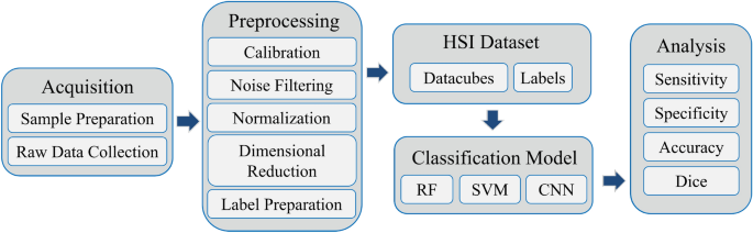
The framework of this study is illustrated in Fig. 1. Initially, we developed a custom hyperspectral microscopy system to acquire raw hyperspectral data from H&E-stained pathological tissue samples. Next, we performed a series of preprocessing steps and label preparation on the hyperspectral data to establish a high-quality hyperspectral dataset. Subsequently, we employed random forest (RF), SVM, 2D CNN, 3D CNN, and an improved hybrid CNN model to identify tumor tissues. Specifically, our improved model, named HybridSN-Att, draws inspiration from the recent work in remote sensing of Roy et al.³⁰, which combines the 2D CNN and 3D CNN to enhance performance.

Biological samples

In this study, ten pathological slides of lung tissue were used, as shown in Fig. 2a. These slides were provided by the State Key Laboratory of Respiratory Disease at the First Affiliated Hospital of Guangzhou Medical University (GMU). We confirm that all methods were performed in accordance with the relevant guidelines and regulations, and the study protocol and procedures were approved by the ethics committee of GMU. The number of Ethics Review Approval Statement is 2022No.163.

All tissue samples underwent a series of standard preparation procedures carried out by professional physicians. The tissues were then stained with H&E. Finally, the entire tissue section was scanned using a digital slide scanner (NanoZoomer S360, Hamamatsu Photonics, Japan) at a magnification of 40x, achieving a pixel-level resolution of 0.23 \(\upmu\)m\(\times\)0.23 \(\upmu\)m. Several pathologists with expertise labeled the digital histological images, as shown in Fig. 2b, primarily outlining the cancer margins of the tissue samples, which included edges between cancerous and normal tissues.

Hyperspectral microscopic collection system setup and characterization

In order to obtain hyperspectral images of lung histopathology sections, we designed an HMI collection system. The physical diagram of the HMI system used in our experiments is shown in Fig. 3a, and the main instruments included a halogen light source (OSL2, 150W, 400-1600nm, Thorlabs Inc., New Jersey, USA), a Complementary Metal Oxide Semiconductor (CMOS) camera (acA3088-57um, Basler Inc., Arensberg, Germany), collimating lens set (AC254-030-AB/AC254-050-AB, Thorlabs Inc., New Jersey, USA), an objective lens (10\(\times\)/0.25, Olympus, Tokyo, Japan) and a liquid crystal tunable filter (LCTF-V10, Wayho Technology Co.). The HMI system has a wavelength range of 420-750 nm, with a total of 67 bands and a spectral resolution of 5 nm. The system is capable of acquiring a set of hyperspectral data in a time frame of less than 20 seconds. The system has a magnification of 10\(\times\), a field of view of 741 \(\upmu\)m \(\times\)495 \(\upmu\)m, and a practical resolution in the range of 1.025–1.830 \(\upmu\)m depending on the light wavelength. Compared with current acquisition devices (see Table 1), the device used in this work has larger resolution and faster scanning speed. Figure. 3b demonstrates the optical collection process of hyperspectral microscopy data. The light from the light source is shaped into parallel light after being transmitted to the collimating lens group through the supporting fiber optic bundle. By continuously adjusting the voltage, the broad-spectrum light is split into a series of narrow spectral bands by the LCTF. This light is then reflected by the beam-splitting prism into the objective lens and focused on the lung histopathology section sample. The reflected light which carries information about the tissue, passed through the beam-splitting prism again and reached the target surface of the CMOS camera after being focused by the tube lens. In this way, we obtained spectral images stored in frequency band order. To prevent interference from external stray light, the experiments conducted in this study were performed in a specific optical darkroom.

Microscopic hyperspectral dataset for pathological sections of lung tissue

In this experiment, within the pathologist-annotated areas of each slide, representative and relatively confidently labeled areas were selected as regions of interest (ROI). Then, these were scanned and collected previously used HMI system. A total of 65 microscopic hyperspectral images were obtained from pathological slides of lung tissues, which were shaped into HMI datacube (specific methods will be detailed in subsequent chapters) and made up the hyperspectral dataset. As illustrated in Fig. 3c, each data cube consists of 67 spectral channels and 3088\(\times\)2064 pixels, with each pixel containing information from all spectral bands. Then, under the guidance of experienced pathologists, these images were annotated, primarily marking the boundaries between the tumor and normal tissues, as well as specifying the locations of some cancer cells. The annotated tumor images were later used for label refinement as described in “Label preparation” section.

Data preprocessing

Hyperspectral data have high dimensionality and are often subject to noise interference from the environment, instruments, and the samples themselves. This complexity makes data processing challenging and time-consuming³⁷. Some studies have shown that data processing difficulties and noise interference can be relieved by applying appropriate preprocessing methods^38,39,40. The data preprocessing pipeline proposed in this research is based on four steps:

Generation of the hyperspectral data cube

Firstly, the continuous single-band images collected from the CMOS detector are stored as multi-band images in Band Sequential Format (BSQ) without undergoing any processing. Subsequently, as depicted in Figure. 3c, we utilize the Python programming language along with its GDAL library⁴¹ to add corresponding parameter information to each band in the stacked multi-band images and transform these into a hyperspectral datacube. Finally, the datacube is stored in RAW file format.

Image calibration

The second step involves the calibration of hyperspectral images. Initially, an area without any tissue on the glass slide is selected as a blank region, and images from this region are captured to serve as the white reference image (\(I_{white}\)). Subsequently, images of the dark noise (\(I_{dark}\)) of the CMOS detector are obtained under no illumination by turning off the light source and covering the objective lens. Calibration aims to eliminate the effects arising from spectral nonuniformity and detector dark current, making it an essential step in the preprocessing of hyperspectral images⁴², as indicated by Equ. (1):

Noise filtering and normalization

The third step involves smoothing all hyperspectral data using the Savitzky-Golay (S-G) algorithm⁴³ (window width is 5 and polynomial order is 2). This process aims to reduce interference from external noise and instrument noise on the HMI system. After smoothing, the hyperspectral data are standardized by the Standard Normal Variate (SNV)⁴⁴, which reduces variability caused by different illumination conditions or sensor settings and allows comparison between different bands. Furthermore, SNV enhances the differences in spectral features between tumor and normal cells, making them more distinguishable from noise and background variation.

Dimensional reduction

The hyperspectral data in this study contain high-dimensional information, which not only increases computational and storage costs but also complicates data analysis and modeling. Dimensionality reduction has proven to be essential for analyzing high-dimensional data⁴⁵, as it removes redundant information and accelerates algorithm execution, thereby enhancing data processing efficiency and model performance. In this work, the principal component analysis (PCA)⁴⁶ method is employed to reduce the dimensionality of the hyperspectral dataset, aiming to improve model accuracy and algorithm speed.

Label preparation

Accurate labeling is crucial in hyperspectral imaging data. Physicians diagnose tumors primarily using cytomorphology³, which provides clear insights into cell structures and tissue. However, the annotation process is often tedious and labor-intensive, leading to coarse labels that can degrade data quality and negatively impact model training. To address this challenge, some studies have manually annotated approximately 10%-20% of the datasets and used these annotations to train network models or experimented with ML methods by randomly selecting a small subset of feature points for testing^47,48. Additionally, some researchers have collaborated with pathologists to comprehensively annotate the entire dataset^28,49,50. Although these methods have shown certain levels of effectiveness, they also come with limitations, such as the risk of overfitting models or the significant human effort and time required-often exceeding 30 minutes per slide. To overcome these issues, we implement a semi-automatic label refinement procedure to reduce data contamination and improve annotation precision, as illustrated in Fig. 4, this procedure requires only 5 minutes to process a single slide. We utilize the K-means unsupervised clustering algorithm to classify hyperspectral data pixels into 20 types based on spectral vectors. A custom interface is used for the manual selection of cell and background regions based on these 20 types. Subsequently, cell regions, background regions and coarse labels are combined together to generate cell-level annotation with four types: non-cell (black), non-tumor cell (green), tumor cell (red), and background (blue). The distinction between non-tumor and tumor cells is guided by tumor annotations provided by pathologists. The resulting classification map is overlaid on the original pathology image for pathologists to verify and adjust. This process improves the accuracy and consistency of the labels, thereby facilitating subsequent analysis and model training.

Supervised classification

The supervised classification algorithms used in this research work include RF, SVM, and CNN, which have been widely used for the classification of hyperspectral images⁵¹. RF is an integrated decision tree-based classifier that aggregates the predictions of multiple decision trees to classify new data. It leverages the uncertainty introduced by randomness to enhance the robustness and generalization of the model³⁶. SVM is a kernel-based supervised classifier. It excels in analyzing high-dimensional feature spaces due to its strong generalization ability and robustness⁵². CNN is a deep learning model widely used in image processing and computer vision. In recent years, researchers have applied CNN to the field of hyperspectral data processing and achieved remarkable results⁵³. Compared with traditional ML algorithms, CNN can effectively utilize spatial and spectral information in hyperspectral data to extract multiscale and multilevel features.

This study proposes a CNN model called HybridSN-Att inspired by recent papers published by Roy et al.³⁰, where the authors proposed a new CNN model for remote sensing image classification. As shown in Fig. 5, the CNN model consists mainly of 3D-CNN and 2D-CNN, where 3D-CNN helps to acquire spatial and spectral features from a set of specific bands, and 2D-CNN effectively extracts the spatial features of hyperspectral images. In addition, we add batch normalization and special convolutional block attention modules in the network structure, including spectral channel attention and spatial attention model, to improve the classification efficiency and generalization ability of the model.